Particle Tracking with PRT
Setup
Packages
from pathlib import Path
import flopy as fp
import numpy as np
import geopandas as gpd
import xarray as xr
import pandas as pd
import matplotlib.pyplot as plt
import matplotlib as mpl

import nlmod
Logging
nlmod.util.get_color_logger("INFO")
nlmod.show_versions()
Python version     : 3.11.14
NumPy version      : 2.4.4
Xarray version     : 2026.4.0
Matplotlib version : 3.10.9
Flopy version      : 3.10.0

nlmod version      : 0.11.3dev
Load base model
model_ws = Path("../examples/00_model_from_scratch")
model_name = "from_scratch"

ds = xr.open_dataset(model_ws / f"{model_name}.nc")
ds.attrs["model_ws"] = model_ws

# constants
wells = pd.DataFrame(
    [[100, -50, -5, -10, -100.0], [200, 150, -20, -30, -300.0]],
    columns=["x", "y", "top", "botm", "Q"],
    index=pd.Index([0, 1], name="well no."),
)
xyriv = [
    (250.0, -500.0),
    (300.0, -300.0),
    (275.0, 0.0),
    (200.0, 250.0),
    (175.0, 500.0),
]
PRT
Forward
# create new subdir for PRT model
prt_ws = Path(model_ws) / "prt_fw"

# Create a new Simulation object
simprt = nlmod.sim.sim(ds, sim_ws=prt_ws)
_ = nlmod.sim.tdis(ds, simprt)

# Add PRT model
prt = nlmod.prt.prt(ds, simprt)

# DIS: discretization package
_ = nlmod.prt.dis(ds, prt)

# MIP: Model Input Package
_ = nlmod.prt.mip(ds, prt, porosity=0.3)

# PRP: particle release point package
# define particle release point  every 11th cell in the first layer
pdata = fp.modpath.ParticleData(
    [
        (k, i, j)
        for i in np.arange(0, ds.sizes["y"], 11)
        for j in np.arange(0, ds.sizes["x"], 11)
        for k in [0]
    ],
    structured=True,
)
release_pts = list(pdata.to_prp(prt.modelgrid, global_xy=False))
prp = nlmod.prt.prp(ds, prt, packagedata=release_pts, perioddata={0: ["FIRST"]})

# FMI: flow model interface
fmi = nlmod.prt.fmi(ds, prt)

# OC: output control
trackcsvfile_prt = f"{prt.name}.trk.csv"
oc = nlmod.prt.oc(
    ds,
    prt,
    trackcsv_filerecord=trackcsvfile_prt,
)

# EMS: explicit model solution
ems = nlmod.sim.ems(simprt, model=prt)
INFO:nlmod.sim.sim.sim:creating mf6 SIM
INFO:nlmod.sim.sim.tdis:creating mf6 TDIS
INFO:nlmod.prt.prt.prt:creating mf6 PRT
INFO:nlmod.gwf.gwf._dis:creating mf6 DIS
INFO:nlmod.prt.prt.mip:creating mf6 MIP
INFO:nlmod.prt.prt.prp:creating mf6 PRP
INFO:nlmod.prt.prt.fmi:creating mf6 FMI
INFO:nlmod.prt.prt.oc:creating mf6 OC
simprt.write_simulation(silent=False)
simprt.run_simulation(silent=False);
writing simulation...
  writing simulation name file...
  writing simulation tdis package...
  writing solution package ems...
  writing model from_scratch_prt...
    writing model name file...
    writing package dis...
    writing package mip...
    writing package prp...
    writing package fmi...
    writing package oc...
FloPy is using the following executable to run the model: ../../../../../../envs/latest/lib/python3.11/site-packages/nlmod/bin/mf6
                                   MODFLOW 6
                U.S. GEOLOGICAL SURVEY MODULAR HYDROLOGIC MODEL
                            VERSION 6.6.3 09/29/2025

   MODFLOW 6 compiled Oct 07 2025 22:51:46 with Intel(R) Fortran Intel(R) 64
   Compiler Classic for applications running on Intel(R) 64, Version 2021.7.0
                             Build 20220726_000000

This software has been approved for release by the U.S. Geological
Survey (USGS). Although the software has been subjected to rigorous
review, the USGS reserves the right to update the software as needed
pursuant to further analysis and review. No warranty, expressed or
implied, is made by the USGS or the U.S. Government as to the
functionality of the software and related material nor shall the
fact of release constitute any such warranty. Furthermore, the
software is released on condition that neither the USGS nor the U.S.
Government shall be held liable for any damages resulting from its
authorized or unauthorized use. Also refer to the USGS Water
Resources Software User Rights Notice for complete use, copyright,
and distribution information.


 MODFLOW runs in SEQUENTIAL mode

 Run start date and time (yyyy/mm/dd hh:mm:ss): 2026/05/13 15:17:28

 Writing simulation list file: mfsim.lst
 Using Simulation name file: mfsim.nam
    Solving:  Stress period:     1    Time step:     1

 Run end date and time (yyyy/mm/dd hh:mm:ss): 2026/05/13 15:17:28
 Elapsed run time:  0.147 Seconds

 Normal termination of simulation.
Load pathline data
The read_pathlines function is a wrapper around pandas.read_csv but it adds the particle id for you. Additionallly it is usefull as documentation on the different istatus and ireason types.
nlmod.prt.read_pathlines?
pathlines_fw = nlmod.prt.read_pathlines(prt_ws / trackcsvfile_prt)
pathlines_fw.head()
| pid | kper | kstp | imdl | iprp | irpt | ilay | icell | izone | istatus | ireason | trelease | t | x | y | z | name | |
|---|---|---|---|---|---|---|---|---|---|---|---|---|---|---|---|---|---|
| 0 | 0 | 1 | 1 | 1 | 1 | 1 | 0 | 0 | 0 | 1 | 0 | 0.0 | 0.000000e+00 | 5.000000 | 995.000000 | -5.000000 | NaN |
| 1 | 0 | 1 | 1 | 1 | 1 | 1 | 0 | 0 | 0 | 1 | 1 | 0.0 | 4.954887e+05 | 1.404571 | 990.000000 | -8.899515 | NaN |
| 2 | 0 | 1 | 1 | 1 | 1 | 1 | 0 | 100 | 0 | 1 | 1 | 0.0 | 5.949531e+05 | 1.096169 | 988.379639 | -10.000000 | NaN |
| 3 | 0 | 1 | 1 | 1 | 1 | 1 | 1 | 10100 | 0 | 1 | 1 | 0.0 | 1.009588e+06 | 1.088284 | 988.279846 | -15.000000 | NaN |
| 4 | 0 | 1 | 1 | 1 | 1 | 1 | 2 | 20100 | 0 | 1 | 1 | 0.0 | 1.097697e+06 | 0.849508 | 980.000000 | -16.053911 | NaN |
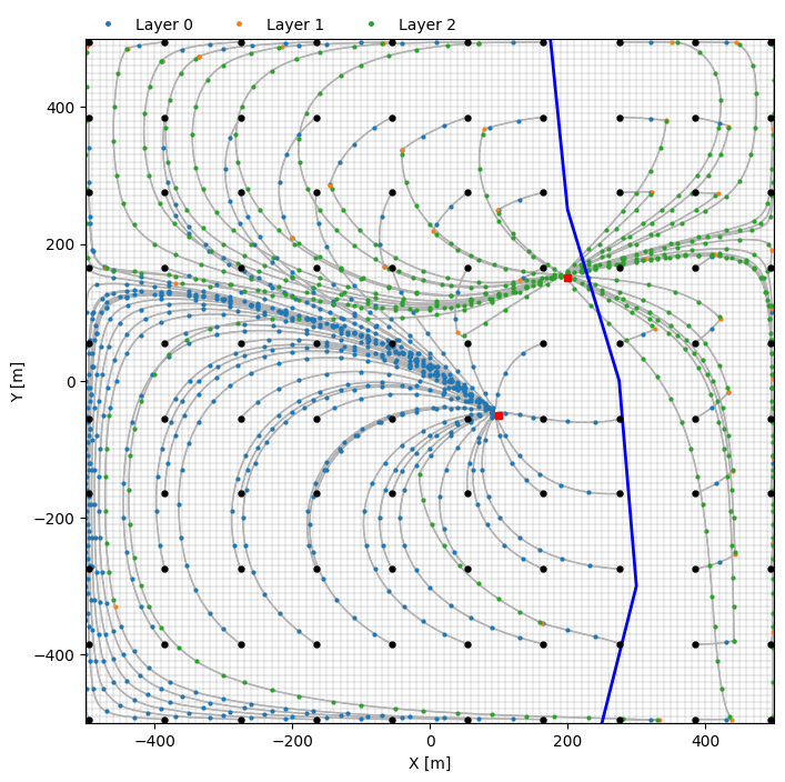
Plot results
f, ax = plt.subplots(figsize=(8, 8))
pmv = fp.plot.PlotMapView(prt, ax=ax)
pmv.plot_grid(lw=0.1, color="k")
pmv.plot_pathline(
    pathlines_fw,
    layer="all",
    colors="0.7",
    lw=1.0,
)
for ilay in [0, 1, 2]:
    mask = pathlines_fw["ilay"] == ilay
    pmv.plot_pathline(
        pathlines_fw.loc[mask],
        layer=ilay - 3,
        lw=0.0,
        marker=".",
        ms=4,
        markercolor=f"C{ilay}",
        markerevery=5,
    )
pmv.plot_endpoint(pathlines_fw, color="k", marker=".", direction="starting", zorder=10)


# plot river and wells
def plot_river_and_wells(ax: plt.Axes):
    ax.plot(
        [xy[0] for xy in xyriv],
        [xy[1] for xy in xyriv],
        "b-",
        lw=2,
        label="river",
    )
    ax.plot(wells["x"].values, wells["y"].values, "rs", ms=5)


plot_river_and_wells(ax=pmv.ax)
handles = [
    pmv.ax.plot([], [], "C0.", ms=5, label="Layer 0")[0],
    pmv.ax.plot([], [], "C1.", ms=5, label="Layer 1")[0],
    pmv.ax.plot([], [], "C2.", ms=5, label="Layer 2")[0],
]
labels = [h.get_label() for h in handles]
pmv.ax.legend(handles, labels, loc=(0, 1), frameon=False, ncol=3)
pmv.ax.set_xlabel("X [m]")
pmv.ax.set_ylabel("Y [m]");
Backward and refined
Refine and run gwf model
refinement_extent = [0.0, 300.0, -100.0, 200.0]
refinement_features = (
    [
        nlmod.util.extent_to_polygon(refinement_extent),
    ],
    "polygon",  # type of feature
    1,  # refinement level
)
dsr = nlmod.grid.refine(ds, refinement_features=[refinement_features])
INFO:nlmod.dims.grid.refine:create vertex grid using gridgen
INFO:nlmod.dims.grid.ds_to_gridprops:resample model Dataset to vertex modelgrid
dsr.attrs["model_name"] = f"{ds.attrs['model_name']}_ref"
dsr.attrs["model_ws"] = f"./{ds.attrs['model_ws']}_ref"
sim = nlmod.sim.sim(dsr)
tdis = nlmod.sim.tdis(dsr, sim)
ims = nlmod.sim.ims(sim, complexity="SIMPLE")
gwf = nlmod.gwf.gwf(dsr, sim)
disv = nlmod.gwf.disv(dsr, gwf)
npf = nlmod.gwf.npf(
    dsr, gwf, save_flows=True, save_specific_discharge=True, save_saturation=True
)
ic = nlmod.gwf.ic(dsr, gwf, starting_head=1.0)
oc = nlmod.gwf.oc(dsr, gwf, save_head=True)
wel = nlmod.gwf.wells.wel_from_df(wells, gwf)

riv_layer = 0  # add to first layer
bed_resistance = 0.1  # days
riv_stage = 1.0  # m NAP
riv_botm = -3.0  # m NAP
riv_data = nlmod.gwf.surface_water.rivdata_from_xylist(
    gwf, xyriv, riv_layer, riv_stage, bed_resistance, riv_botm
)


def get_riv_cond_from_cid(icell2d: int, ds: xr.Dataset, bed_resistance: float) -> float:
    """Get river conductance from cell id."""
    area = ds.area.sel(icell2d=icell2d).values
    # calculate conductance
    return area / bed_resistance


riv_datac = [
    [x[0], x[1], get_riv_cond_from_cid(x[0][1], dsr, x[2]), x[3]] for x in riv_data
]
riv = fp.mf6.ModflowGwfriv(gwf, stress_period_data={0: riv_datac})

nlmod.sim.write_and_run(sim, dsr, silent=False)
INFO:nlmod.sim.sim.sim:creating mf6 SIM
INFO:nlmod.sim.sim.tdis:creating mf6 TDIS
INFO:nlmod.sim.sim.ims:creating mf6 IMS
INFO:nlmod.gwf.gwf.gwf:creating mf6 GWF
INFO:nlmod.gwf.gwf._disv:creating mf6 DISV
INFO:nlmod.gwf.gwf.npf:creating mf6 NPF
INFO:nlmod.gwf.gwf.ic:creating mf6 IC
INFO:nlmod.gwf.gwf.ic:adding 'starting_head' data array to ds
INFO:nlmod.gwf.gwf.oc:creating mf6 OC
INFO:nlmod.sim.sim.write_and_run:write model dataset to cache
INFO:nlmod.sim.sim.write_and_run:write modflow files to model workspace
writing simulation...
  writing simulation name file...
  writing simulation tdis package...
  writing solution package ims...
  writing model from_scratch_ref...
    writing model name file...
    writing package disv...
    writing package npf...
    writing package ic...
    writing package oc...
    writing package wel_0...
INFORMATION: maxbound in ('', 'wel', 'dimensions') changed to 2 based on size of stress_period_data
    writing package riv_0...
INFORMATION: maxbound in ('', 'riv', 'dimensions') changed to 139 based on size of stress_period_data
INFO:nlmod.sim.sim.write_and_run:run model
FloPy is using the following executable to run the model: ../../../../../envs/latest/lib/python3.11/site-packages/nlmod/bin/mf6
                                   MODFLOW 6
                U.S. GEOLOGICAL SURVEY MODULAR HYDROLOGIC MODEL
                            VERSION 6.6.3 09/29/2025

   MODFLOW 6 compiled Oct 07 2025 22:51:46 with Intel(R) Fortran Intel(R) 64
   Compiler Classic for applications running on Intel(R) 64, Version 2021.7.0
                             Build 20220726_000000

This software has been approved for release by the U.S. Geological
Survey (USGS). Although the software has been subjected to rigorous
review, the USGS reserves the right to update the software as needed
pursuant to further analysis and review. No warranty, expressed or
implied, is made by the USGS or the U.S. Government as to the
functionality of the software and related material nor shall the
fact of release constitute any such warranty. Furthermore, the
software is released on condition that neither the USGS nor the U.S.
Government shall be held liable for any damages resulting from its
authorized or unauthorized use. Also refer to the USGS Water
Resources Software User Rights Notice for complete use, copyright,
and distribution information.


 MODFLOW runs in SEQUENTIAL mode

 Run start date and time (yyyy/mm/dd hh:mm:ss): 2026/05/13 15:17:34

 Writing simulation list file: mfsim.lst
 Using Simulation name file: mfsim.nam

    Solving:  Stress period:     1    Time step:     1

 Run end date and time (yyyy/mm/dd hh:mm:ss): 2026/05/13 15:17:35
 Elapsed run time:  0.463 Seconds

 Normal termination of simulation.
Intersecting with grid:   0%|          | 0/2 [00:00<?, ?it/s]
Intersecting with grid: 100%|██████████| 2/2 [00:00<00:00, 283.25it/s]
Reverse heads and cellbudget files
hds = nlmod.gwf.get_headfile(ds=dsr, gwf=gwf, tdis=tdis)
hds_bw_path = hds.filename.parent / f"{hds.filename.stem}_bkwd{hds.filename.suffix}"
hds.reverse(hds_bw_path)

cbc = nlmod.gwf.get_cellbudgetfile(ds=dsr, gwf=gwf, tdis=tdis)
cbc_bw_path = cbc.filename.parent / f"{cbc.filename.stem}_bkwd{cbc.filename.suffix}"
cbc.reverse(cbc_bw_path)
Create particle starts list
Start a particle in each (active) cell in refined extent
dsr["z"] = (dsr["top"] + dsr["botm"]) / 2
dsr["idomain"] = (
    ("layer", "icell2d"),
    disv.idomain.array,
)  # make sure to get idomain otherwhise you might start particles in inactive cells and everything crashes #beentheredonethat

# map xy to cellids
nodes = dsr[["z", "idomain"]].where(
    (dsr.x >= refinement_extent[0])
    & (dsr.x <= refinement_extent[1])
    & (dsr.y >= refinement_extent[2])
    & (dsr.y <= refinement_extent[3]),
    drop=True,
)
ix = fp.utils.GridIntersect(gwf.modelgrid)
spatial_join = gpd.GeoDataFrame(
    geometry=gpd.points_from_xy(nodes.x, nodes.y),
).sjoin(
    gpd.GeoDataFrame(
        {"cellid": ix.cellids},
        geometry=ix.geoms,
    ),
    how="left",
)

# create release points
# define particle release point for every cell within refined extent
pid = 0
release_pts = []
for ilay in range(nodes.sizes["layer"]):
    nodes_lay = nodes.isel(layer=ilay)
    active = (nodes_lay["idomain"] > 0).values
    j = spatial_join["cellid"].values.astype(int)[active]
    k = np.full_like(j, ilay, dtype=int)
    x = nodes_lay["x"].values[active]
    y = nodes_lay["y"].values[active]
    z = nodes_lay["z"].values[active]
    pids = np.arange(pid, pid + len(k), dtype=int)
    pid += len(k)
    cellid = tuple(zip(k, j))
    release_ptsi = list(zip(pids, cellid, x, y, z))
    release_pts += release_ptsi

print(f"Number of release points: {len(release_pts)}")
Number of release points: 10800
# create new subdir for PRT backwards model
prt_ws_bw = Path(dsr.attrs["model_ws"]) / "prt_bw"

# Create a new Simulation object
simprt_bw = nlmod.sim.sim(dsr, sim_ws=prt_ws_bw)
_ = nlmod.sim.tdis(dsr, simprt_bw)

# Add PRT model
prt_bw = nlmod.prt.prt(dsr, simprt_bw, modelname=dsr.model_name)

# Add DISV model
_ = nlmod.prt.disv(dsr, prt_bw)

# MIP: Model Input Package
_ = nlmod.prt.mip(dsr, prt_bw, porosity=0.3)

# PRP: particle release package
_ = nlmod.prt.prp(
    dsr,
    prt_bw,
    packagedata=release_pts,
    perioddata={0: ["FIRST"]},
)

# OC: output control
trackcsvfile_prt_bw = f"{prt_bw.name}bw.trk.csv"
_ = nlmod.prt.oc(dsr, prt_bw, trackcsv_filerecord=trackcsvfile_prt_bw)

# FMI: flow model interface
fmi_bw_packagedata = [
    ("GWFHEAD", hds_bw_path),
    ("GWFBUDGET", cbc_bw_path),
]
_ = nlmod.prt.fmi(dsr, prt_bw, packagedata=fmi_bw_packagedata)

# EMS: explicit model solution
_ = nlmod.sim.ems(simprt_bw, model=prt_bw)

# Write and run the simulation
simprt_bw.write_simulation()
success_bw_prt, _ = simprt_bw.run_simulation()
INFO:nlmod.sim.sim.sim:creating mf6 SIM
INFO:nlmod.sim.sim.tdis:creating mf6 TDIS
INFO:nlmod.prt.prt.prt:creating mf6 PRT
INFO:nlmod.gwf.gwf._disv:creating mf6 DISV
INFO:nlmod.prt.prt.mip:creating mf6 MIP
INFO:nlmod.prt.prt.prp:creating mf6 PRP
INFO:nlmod.prt.prt.oc:creating mf6 OC
INFO:nlmod.prt.prt.fmi:creating mf6 FMI
writing simulation...
  writing simulation name file...
  writing simulation tdis package...
  writing solution package ems...
  writing model from_scratch_ref...
    writing model name file...
    writing package disv...
    writing package mip...
    writing package prp...
    writing package oc...
    writing package fmi...
FloPy is using the following executable to run the model: ../../../../../../envs/latest/lib/python3.11/site-packages/nlmod/bin/mf6
                                   MODFLOW 6
                U.S. GEOLOGICAL SURVEY MODULAR HYDROLOGIC MODEL
                            VERSION 6.6.3 09/29/2025

   MODFLOW 6 compiled Oct 07 2025 22:51:46 with Intel(R) Fortran Intel(R) 64
   Compiler Classic for applications running on Intel(R) 64, Version 2021.7.0
                             Build 20220726_000000

This software has been approved for release by the U.S. Geological
Survey (USGS). Although the software has been subjected to rigorous
review, the USGS reserves the right to update the software as needed
pursuant to further analysis and review. No warranty, expressed or
implied, is made by the USGS or the U.S. Government as to the
functionality of the software and related material nor shall the
fact of release constitute any such warranty. Furthermore, the
software is released on condition that neither the USGS nor the U.S.
Government shall be held liable for any damages resulting from its
authorized or unauthorized use. Also refer to the USGS Water
Resources Software User Rights Notice for complete use, copyright,
and distribution information.


 MODFLOW runs in SEQUENTIAL mode

 Run start date and time (yyyy/mm/dd hh:mm:ss): 2026/05/13 15:17:36

 Writing simulation list file: mfsim.lst
 Using Simulation name file: mfsim.nam

    Solving:  Stress period:     1    Time step:     1

 Run end date and time (yyyy/mm/dd hh:mm:ss): 2026/05/13 15:17:42
 Elapsed run time:  5.590 Seconds

 Normal termination of simulation.
Load pathline data
pathlines_bw = nlmod.prt.read_pathlines(
    prt_ws_bw / trackcsvfile_prt_bw, icell2d=dsr.icell2d.size
)
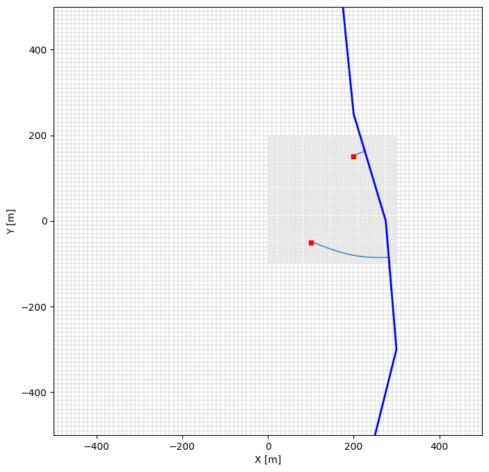
Get pathlines of particles that started in a well (backward)
pathlines_bw0 = pathlines_bw.query("ireason==0")
well_pids = []
for _, row in wel.stress_period_data.dataframe[0].iterrows():
    cellid_layer = row["cellid_layer"]
    icell2d = row["cellid_cell"]
    well_pids.append(
        pathlines_bw0.query(f"ilay=={cellid_layer} and icell2d=={icell2d}")
        .loc[:, "pid"]
        .to_numpy()[0]
    )
pathlines_bww = pathlines_bw[pathlines_bw["pid"].isin(well_pids)]
Plot results
f, ax = plt.subplots(figsize=(8, 8))
for pid, gr in pathlines_bww.groupby("pid"):
    for ilay, gr_lay in gr.groupby("ilay"):
        ax.plot(gr_lay["x"], gr_lay["y"], lw=1.0, color=f"C{ilay}", zorder=1)

nlmod.plot.modelgrid(dsr, ax=ax, linewidth=0.1)
plot_river_and_wells(ax=ax)
ax.set_xlim(ds.extent[0], ds.extent[1])
ax.set_ylim(ds.extent[2], ds.extent[3])
ax.set_aspect("equal")
ax.set_xlabel("X [m]")
_ = ax.set_ylabel("Y [m]")
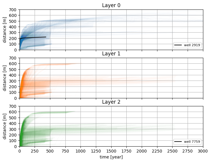
f, axes = plt.subplots(3, 1, figsize=(8, 6), sharex=True, sharey=True)

for pid, gr in pathlines_bw.groupby("pid"):
    t0 = gr["t"].idxmin()
    x0, y0, z0, ilay0 = gr.loc[t0, ["x", "y", "z", "ilay"]]
    distance = np.sqrt((gr["x"] - x0) ** 2 + (gr["y"] - y0) ** 2 + (gr["z"] - z0) ** 2)
    if pid in well_pids:
        plot_kwargs = {"color": "k", "alpha": 1.0, "zorder": 10, "label": f"well {pid}"}
    else:
        plot_kwargs = {"color": f"C{ilay0}", "alpha": 0.01}
    axes[ilay0].plot(gr["t"] / 365.25, distance, **plot_kwargs)

for i, ax in enumerate(axes):
    ax.xaxis.set_major_locator(mpl.ticker.MultipleLocator(250))
    ax.yaxis.set_major_locator(mpl.ticker.MultipleLocator(100))
    ax.set_ylabel("distance [m]")
    ax.set_title(f"Layer {i}")
    ax.grid(True)
    handles, labels = ax.get_legend_handles_labels()
    if labels:
        ax.legend(handles, labels, loc="lower right", ncol=1, fontsize=8, frameon=True)
    ax.set_xlim(0.0, 3000.0)
    ax.set_ylim(0.0, 700.0)
_ = axes[-1].set_xlabel("time [year]")