Working with grid rotation
Rotated grids are supported in nlmod. It is implemented in the following manner:
angrot,xoriginandyorigin(naming identical to modflow 6) are added to the attributes of the model Dataset.angrotis the counter-clockwise rotation angle (in degrees) of the model grid coordinate system relative to a real-world coordinate system (identical to definition in modflow 6)when a grid is rotated:
xandy(andxvandyvfor a vertex grid) are in model coordinates, instead of real-world coordinates.xcandycare added to the Dataset and represent the cell centers in real-world coordinates (naming identical to rioxarray rotated grids)the plot-methods in nlmod plot the grid in model coordinates by default (can be overridden by the setting the parameter
rotated=True)before intersecting with the grid, GeoDataFrames are automatically transformed to model coordinates.
When grids are not rotated, the model Dataset does not contain an attribute named angrot (or it is 0). The x- and y-coordinates of the model then respresent real-world coordinates.
In this notebook we generate a model of 1 by 1 km, with a grid that is rotated 10 degrees relative to the real-world coordinates system (EPSG:28992: RD-coordinates).
import os

import matplotlib

import nlmod
nlmod.util.get_color_logger("INFO")
nlmod.show_versions()
Python version     : 3.11.14
NumPy version      : 2.4.4
Xarray version     : 2026.4.0
Matplotlib version : 3.10.9
Flopy version      : 3.10.0

nlmod version      : 0.11.3dev
Generate a model Dataset
We generate a model dataset with a rotation of 10 degrees counterclockwise.
ds = nlmod.get_ds(
    [0, 1000, 0, 1000],
    angrot=10.0,
    xorigin=200_000,
    yorigin=500_000,
    delr=10.0,
    model_name="nlmod",
    model_ws="02_grid_rotation",
)

ds = nlmod.time.set_ds_time(ds, time="2023-01-01", start="2013-01-01")
INFO:nlmod.dims.base.to_model_ds:resample layer model data to structured modelgrid
Use a disv-grid
We call the refine method to generate a vertex grid (with the option of grid-refinement), instead of a structured grid. We can comment the next line to model a structured grid, and the rest of the notebook will run without problems as well.
ds = nlmod.grid.refine(ds)
INFO:nlmod.dims.grid.refine:create vertex grid using gridgen
INFO:nlmod.dims.grid.ds_to_gridprops:resample model Dataset to vertex modelgrid
Add AHN
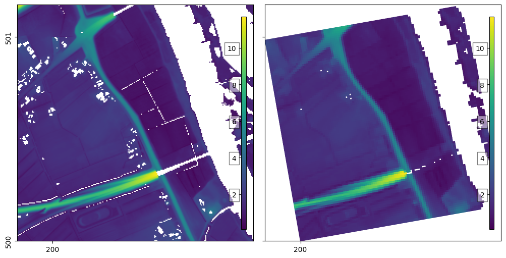
Download the ahn, resample to the new grid (using the method ‘average’) and compare.
# Download AHN
extent = nlmod.grid.get_extent(ds)
ahn = nlmod.read.ahn.download_ahn3(extent)

# Resample to the grid
ds["ahn"] = nlmod.resample.structured_da_to_ds(ahn, ds, method="average")

# Compare original ahn to the resampled one
f, axes = nlmod.plot.get_map(extent, ncols=2)
norm = matplotlib.colors.Normalize()
pc = nlmod.plot.data_array(ahn, ax=axes[0], norm=norm)
nlmod.plot.colorbar_inside(pc, ax=axes[0])
pc = nlmod.plot.data_array(
    ds["ahn"], ds=ds, ax=axes[1], rotated=True, norm=norm, edgecolor="face"
)
nlmod.plot.colorbar_inside(pc, ax=axes[1]);
Downloading tiles of AHN3:   0%|          | 0/2 [00:00<?, ?it/s]
Downloading tiles of AHN3: 100%|██████████| 2/2 [00:02<00:00,  1.45s/it]
Download surface water
Download BGT-polygon data, add stage information from the waterboard, and grid the polygons. Because we use a rotated grid, the bgt-polygons are in model coordinates.
bgt = nlmod.read.bgt.download_bgt(extent)
bgt = nlmod.gwf.surface_water.add_stages_from_waterboards(bgt, extent=extent)
bgt = nlmod.grid.gdf_to_grid(bgt, ds).set_index("cellid")
INFO:nlmod.gwf.surface_water.download_level_areas:Downloading level_areas for Vallei en Veluwe
INFO:nlmod.gwf.surface_water.download_level_areas:Downloading level_areas for Vallei & Veluwe
Adding ['summer_stage', 'winter_stage'] from Vallei en Veluwe:   0%|          | 0/129 [00:00<?, ?it/s]
Adding ['summer_stage', 'winter_stage'] from Vallei en Veluwe: 100%|██████████| 129/129 [00:00<00:00, 961.53it/s]
Adding ['summer_stage', 'winter_stage'] from Vallei & Veluwe:   0%|          | 0/129 [00:00<?, ?it/s]
Adding ['summer_stage', 'winter_stage'] from Vallei & Veluwe: 100%|██████████| 129/129 [00:00<00:00, 969.77it/s]
Intersecting with grid:   0%|          | 0/159 [00:00<?, ?it/s]
Intersecting with grid: 100%|██████████| 159/159 [00:01<00:00, 79.59it/s]
Download knmi-data
knmi_ds = nlmod.read.knmi.get_recharge(ds)
ds.update(knmi_ds)
INFO:hydropandas.io.knmi.get_knmi_obs:get data from station 302 and variable RD from 2013-01-01 to 2023-01-01
INFO:hydropandas.io.knmi.fill_missing_measurements:station 302 has no measurements between 2013-01-01 00:00:00 and 2023-01-01 00:00:00 trying to get measurements from nearest station -> 329
INFO:hydropandas.io.knmi.get_knmi_obs:get data from station 278 and variable EV24 from 2013-01-01 to 2023-01-01
WARNING:nlmod.read.knmi.discretize_knmi:The default of hourly_precision=False will be changed to True in a future version of nlmod. Pass hourly_precision=False to retain current behavior or hourly_precision=True to adopt the future default and silence this warning.
Generate flopy-model
We generate a simulation and a groundwater flow model, with some standard packages.
# %%
# create simulation
sim = nlmod.sim.sim(ds)

# create time discretisation
tdis = nlmod.sim.tdis(ds, sim)

# create ims
ims = nlmod.sim.ims(sim, complexity="complex")

# create groundwater flow model
gwf = nlmod.gwf.gwf(ds, sim)

# Create discretization
dis = nlmod.gwf.dis(ds, gwf)

# create node property flow
npf = nlmod.gwf.npf(ds, gwf)

# Create the initial conditions package
ic = nlmod.gwf.ic(ds, gwf, starting_head=0.0)

# Create the output control package
oc = nlmod.gwf.oc(ds, gwf)

# create recharge package
rch = nlmod.gwf.rch(ds, gwf)
INFO:nlmod.sim.sim.sim:creating mf6 SIM
INFO:nlmod.sim.sim.tdis:creating mf6 TDIS
INFO:nlmod.sim.sim.ims:creating mf6 IMS
INFO:nlmod.gwf.gwf.gwf:creating mf6 GWF
INFO:nlmod.gwf.gwf._disv:creating mf6 DISV
INFO:nlmod.gwf.gwf.npf:creating mf6 NPF
INFO:nlmod.gwf.gwf.ic:creating mf6 IC
INFO:nlmod.gwf.gwf.ic:adding 'starting_head' data array to ds
INFO:nlmod.gwf.gwf.oc:creating mf6 OC
INFO:nlmod.gwf.gwf.rch:creating mf6 RCH
Add surface water
To the groundwater flow model
# add surface water with a winter and a summer stage
# (which are both added with about half their conductance in a steady state simulation)
drn = nlmod.gwf.surface_water.gdf_to_seasonal_pkg(bgt, gwf, ds, print_input=True)
INFO:nlmod.gwf.surface_water.gdf_to_seasonal_pkg:Filling 3364 NaN's in rbot using a water depth of 0.5 meter.
INFO:nlmod.gwf.surface_water.gdf_to_seasonal_pkg:Calcluating DRN-conductance based on as resistance of 1.0 days.
WARNING:nlmod.gwf.surface_water.build_spd:2038 records without a stage ignored
WARNING:nlmod.gwf.surface_water.build_spd:2038 records without a stage ignored
Building stress period data for winter DRN:   0%|          | 0/1326 [00:00<?, ?it/s]
Building stress period data for winter DRN: 100%|██████████| 1326/1326 [00:00<00:00, 7727.27it/s]
Building stress period data for summer DRN:   0%|          | 0/1326 [00:00<?, ?it/s]
Building stress period data for summer DRN: 100%|██████████| 1326/1326 [00:00<00:00, 7826.76it/s]
Run the model and read the heads
# run the model
nlmod.sim.write_and_run(sim, ds)

# read the heads
head = nlmod.gwf.get_heads_da(ds)
INFO:nlmod.sim.sim.write_and_run:write model dataset to cache
INFO:nlmod.sim.sim.write_and_run:write modflow files to model workspace
writing simulation...
  writing simulation name file...
  writing simulation tdis package...
  writing solution package ims...
  writing model nlmod...
    writing model name file...
    writing package disv...
    writing package npf...
    writing package ic...
    writing package oc...
    writing package rch...
    writing package drn_0...
INFORMATION: maxbound in ('', 'drn', 'dimensions') changed to 2652 based on size of stress_period_data
    writing package obs_0...
    writing package ts_0...
INFO:nlmod.sim.sim.write_and_run:run model
FloPy is using the following executable to run the model: ../../../../../envs/latest/lib/python3.11/site-packages/nlmod/bin/mf6
                                   MODFLOW 6
                U.S. GEOLOGICAL SURVEY MODULAR HYDROLOGIC MODEL
                            VERSION 6.6.3 09/29/2025

   MODFLOW 6 compiled Oct 07 2025 22:51:46 with Intel(R) Fortran Intel(R) 64
   Compiler Classic for applications running on Intel(R) 64, Version 2021.7.0
                             Build 20220726_000000

This software has been approved for release by the U.S. Geological
Survey (USGS). Although the software has been subjected to rigorous
review, the USGS reserves the right to update the software as needed
pursuant to further analysis and review. No warranty, expressed or
implied, is made by the USGS or the U.S. Government as to the
functionality of the software and related material nor shall the
fact of release constitute any such warranty. Furthermore, the
software is released on condition that neither the USGS nor the U.S.
Government shall be held liable for any damages resulting from its
authorized or unauthorized use. Also refer to the USGS Water
Resources Software User Rights Notice for complete use, copyright,
and distribution information.


 MODFLOW runs in SEQUENTIAL mode

 Run start date and time (yyyy/mm/dd hh:mm:ss): 2026/05/13 15:16:13

 Writing simulation list file: mfsim.lst
 Using Simulation name file: mfsim.nam
    Solving:  Stress period:     1    Time step:     1

 Run end date and time (yyyy/mm/dd hh:mm:ss): 2026/05/13 15:16:14
 Elapsed run time:  0.582 Seconds

 Normal termination of simulation.
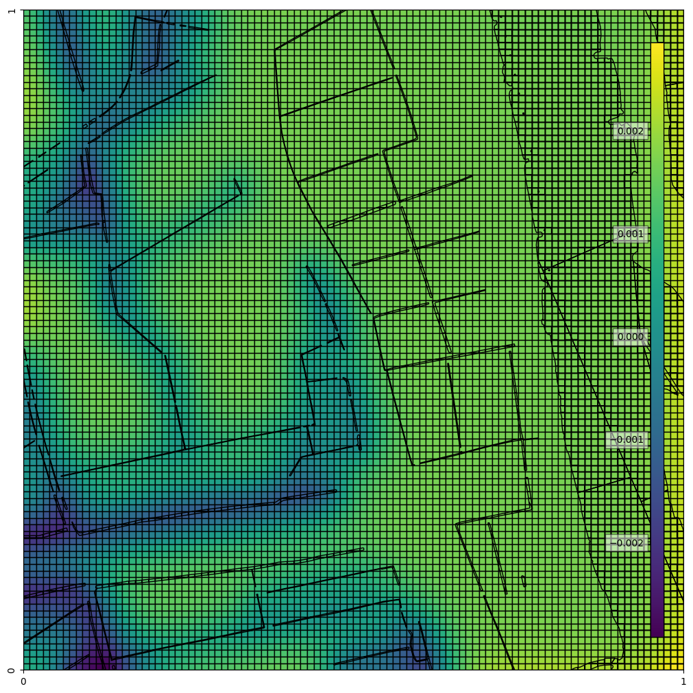
Plot the heads in layer 1
When grid rotation is used, nlmod.plot.data_array() plots a DataArray in model coordinates.
f, ax = nlmod.plot.get_map(ds.extent)
pc = nlmod.plot.data_array(head.sel(layer=1).mean("time"), ds=ds, edgecolor="k")
cbar = nlmod.plot.colorbar_inside(pc)
bgt.plot(ax=ax, edgecolor="k", facecolor="none")
<Axes: >
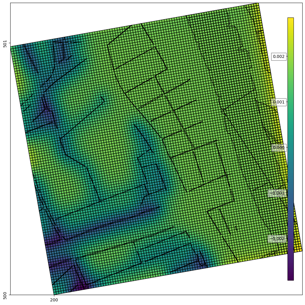
If we want to plot in realworld coordinates, we set the optional parameter rotated=True.
f, ax = nlmod.plot.get_map(extent)
pc = nlmod.plot.data_array(
    head.sel(layer=1).mean("time"), ds=ds, edgecolor="k", rotated=True
)
cbar = nlmod.plot.colorbar_inside(pc)
# as the surface water shapes are in model coordinates, we need to transform them
# to real-world coordinates before plotting
affine = nlmod.grid.get_affine_mod_to_world(ds)
bgt_rw = nlmod.grid.affine_transform_gdf(bgt, affine)
bgt_rw.plot(ax=ax, edgecolor="k", facecolor="none")
<Axes: >
Export the model dataset to a netcdf-file, which you can open in qgis using ‘Add mesh layer’.
fname = os.path.join(ds.model_ws, "ugrid_ds.nc")
nlmod.gis.ds_to_ugrid_nc_file(ds, fname)
<xarray.Dataset> Size: 4MB
Dimensions:          (icell2d: 10000, time: 1, iv: 10201, icv: 4)
Coordinates:
    xc               (icell2d) float64 80kB 1.998e+05 1.998e+05 ... 2.01e+05
    yc               (icell2d) float64 80kB 5.01e+05 5.01e+05 ... 5.002e+05
    x                (icell2d) float64 80kB 5.0 15.0 25.0 ... 975.0 985.0 995.0
    y                (icell2d) float64 80kB 995.0 995.0 995.0 ... 5.0 5.0 5.0
  * time             (time) datetime64[ns] 8B 2023-01-01
    spatial_ref      int64 8B 0
Dimensions without coordinates: icell2d, iv, icv
Data variables: (12/51)
    top              (icell2d) float64 80kB 0.0 0.0 0.0 0.0 ... 0.0 0.0 0.0 0.0
    botm_0           (icell2d) float64 80kB -10.0 -10.0 -10.0 ... -10.0 -10.0
    botm_1           (icell2d) float64 80kB -20.0 -20.0 -20.0 ... -20.0 -20.0
    botm_2           (icell2d) float64 80kB -30.0 -30.0 -30.0 ... -30.0 -30.0
    botm_3           (icell2d) float64 80kB -40.0 -40.0 -40.0 ... -40.0 -40.0
    botm_4           (icell2d) float64 80kB -50.0 -50.0 -50.0 ... -50.0 -50.0
    ...               ...
    starting_head_5  (icell2d) float64 80kB 0.0 0.0 0.0 0.0 ... 0.0 0.0 0.0 0.0
    starting_head_6  (icell2d) float64 80kB 0.0 0.0 0.0 0.0 ... 0.0 0.0 0.0 0.0
    starting_head_7  (icell2d) float64 80kB 0.0 0.0 0.0 0.0 ... 0.0 0.0 0.0 0.0
    starting_head_8  (icell2d) float64 80kB 0.0 0.0 0.0 0.0 ... 0.0 0.0 0.0 0.0
    starting_head_9  (icell2d) float64 80kB 0.0 0.0 0.0 0.0 ... 0.0 0.0 0.0 0.0
    mesh_topology    int64 8B 0
Attributes: (12/16)
    extent:                            [0, 1000, 0, 1000]
    xorigin:                           200000
    yorigin:                           500000
    angrot:                            10.0
    gridtype:                          vertex
    model_name:                        nlmod
    ...                                ...
    figdir:                            02_grid_rotation/figure
    cachedir:                          02_grid_rotation/cache
    transport:                         0
    model_dataset_written_to_disk_on:  20260513_15:16:12
    model_data_written_to_disk_on:     20260513_15:16:13
    model_ran_on:                      20260513_15:16:14