Using information from GeoTOP
Most geohydrological models in the Netherlands use the layer model REGIS as the basis for the geohydrological properties of the model. However, REGIS does not contain information for all layers, of which the holocene confining layer (HLc) is the most important one. In this notebook we will show how to use the voxel model GeoTOP to generate geohydrolocal properties for this layer.
import numpy as np
import matplotlib
import matplotlib.pyplot as plt
from shapely.geometry import LineString

import nlmod
nlmod.util.get_color_logger("INFO")
nlmod.show_versions()
Python version     : 3.11.14
NumPy version      : 2.4.4
Xarray version     : 2026.4.0
Matplotlib version : 3.10.9
Flopy version      : 3.10.0

nlmod version      : 0.11.3dev
# Define an extent and a line from southwest to northeast through this extent
extent = [100000.0, 105000.0, 499800.0, 500000.0]
line = LineString([(extent[0], extent[2]), (extent[1], extent[3])])
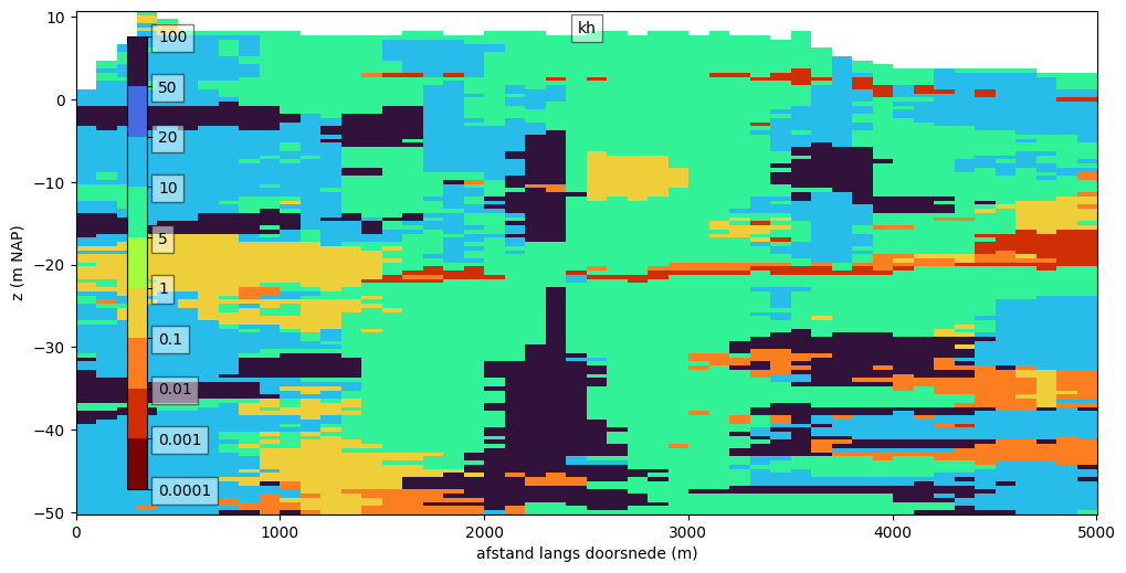
We define a method called ‘plot_kh_kv’, which we can call in cells below to plot the horizontal and vertical conductivity in a cross-section.
def plot_kh_kv(
    ds,
    layer="layer",
    variables=None,
    zmin=-50.25,
    min_label_area=None,
    cmap=None,
    norm=None,
):
    if variables is None:
        variables = ["kh", "kv"]
    if cmap is None:
        cmap = plt.get_cmap("turbo_r")
    if norm is None:
        boundaries = [0.0001, 0.001, 0.01, 0.1, 1, 5, 10, 20, 50, 100]
        norm = matplotlib.colors.BoundaryNorm(boundaries, cmap.N)
    for var in variables:
        f, ax = plt.subplots(figsize=(10, 5))
        cs = nlmod.plot.DatasetCrossSection(ds, line, layer=layer, ax=ax, zmin=zmin)
        pc = cs.plot_array(ds[var], norm=norm, cmap=cmap)
        if min_label_area is not None:
            cs.plot_layers(alpha=0.0, min_label_area=min_label_area)
            cs.plot_grid(vertical=False)
        format = matplotlib.ticker.FuncFormatter(lambda y, _: "{:g}".format(y))
        nlmod.plot.colorbar_inside(pc, bounds=[0.05, 0.05, 0.02, 0.9], format=format)
        nlmod.plot.title_inside(var, ax=ax)
        ax.set_xlabel("afstand langs doorsnede (m)")
        ax.set_ylabel("z (m NAP)")
        f.tight_layout(pad=0.0)
Download GeoTOP
We download GeoTOP for a certain extent. We get an xarray.Dataset with voxels of 100 * 100 * 0.5 (dx * dy * dz) m, with variables ‘strat’ and ‘lithok’. We also get the probaliblity of the occurence of each lithoclass in variables named ‘kans_*’ (since we set probabilities=True).
gt = nlmod.read.geotop.download_geotop(extent, probabilities=True)
gt
<xarray.Dataset> Size: 2MB
Dimensions: (z: 313, y: 2, x: 50)
Coordinates:
* z (z) float32 1kB 106.0 105.5 105.0 104.5 ... -48.5 -49.0 -49.5 -50.0
* y (y) float64 16B 5e+05 4.998e+05
* x (x) float64 400B 1e+05 1.002e+05 1.002e+05 ... 1.048e+05 1.05e+05
Data variables: (12/13)
strat (z, y, x) float32 125kB dask.array<chunksize=(9, 2, 50), meta=np.ndarray>
lithok (z, y, x) float32 125kB dask.array<chunksize=(9, 2, 50), meta=np.ndarray>
kans_1 (z, y, x) float32 125kB dask.array<chunksize=(9, 2, 50), meta=np.ndarray>
kans_2 (z, y, x) float32 125kB dask.array<chunksize=(9, 2, 50), meta=np.ndarray>
kans_3 (z, y, x) float32 125kB dask.array<chunksize=(9, 2, 50), meta=np.ndarray>
kans_4 (z, y, x) float32 125kB dask.array<chunksize=(9, 2, 50), meta=np.ndarray>
... ...
kans_6 (z, y, x) float32 125kB dask.array<chunksize=(9, 2, 50), meta=np.ndarray>
kans_7 (z, y, x) float32 125kB dask.array<chunksize=(9, 2, 50), meta=np.ndarray>
kans_8 (z, y, x) float32 125kB dask.array<chunksize=(9, 2, 50), meta=np.ndarray>
kans_9 (z, y, x) float32 125kB dask.array<chunksize=(9, 2, 50), meta=np.ndarray>
onz_lk (z, y, x) float32 125kB dask.array<chunksize=(9, 2, 50), meta=np.ndarray>
onz_ls (z, y, x) float32 125kB dask.array<chunksize=(9, 2, 50), meta=np.ndarray>
Attributes:
title: geotop v01r6s1 (100.0m * 100.0m * 0.5m
references: http://www.dinoloket.nl/detaillering-van-de-bovenste-lagen...
comment: GeoTOP 1.6.1 (lithoklasse)
disclaimer: http://www.dinoloket.nl
terms_of_use: http://www.dinoloket.nl
institution: TNO / Geologische Dienst Nederland
Conventions: CF-1.4
source: Generated by nl.tno.dino.geo3dmodel.generator.GeoTOPVoxelM...
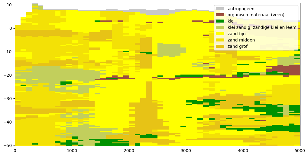
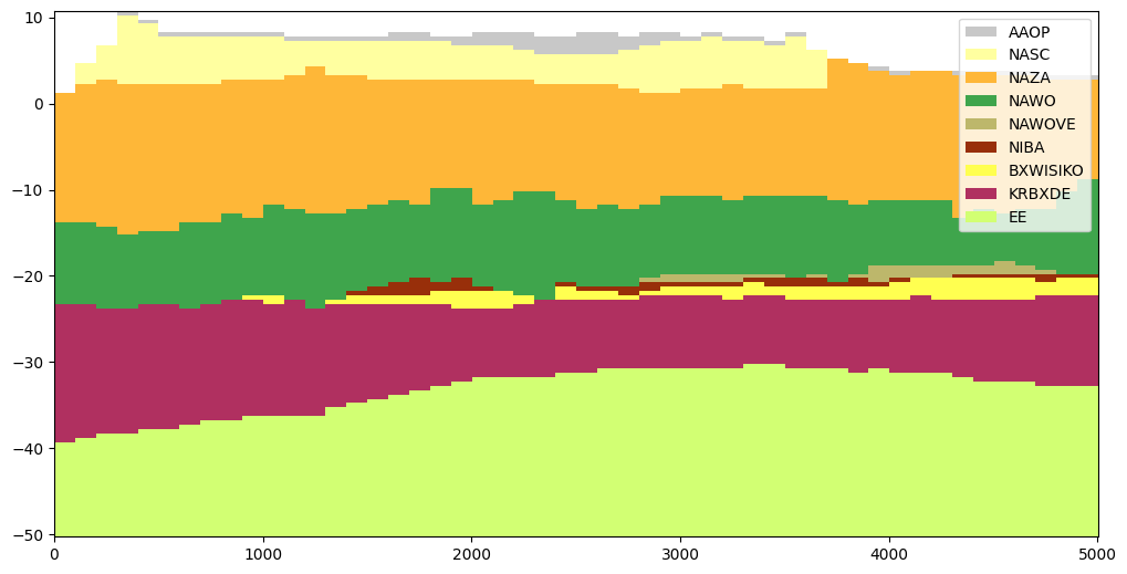
history: Generated on Thu May 01 22:54:36 CEST 2025We plot the lithoclass (soil types) and the stratigraphy (geological units) in two cross-sections using the methods nlmod.plot.geotop_lithok_in_cross_section & nlmod.plot.geotop_strat_in_cross_section.
f, ax = plt.subplots(figsize=(10, 5))
nlmod.plot.geotop_lithok_in_cross_section(line, gt)
f.tight_layout(pad=0.0)
f, ax = plt.subplots(figsize=(10, 5))
nlmod.plot.geotop_strat_in_cross_section(line, gt, ax=ax)
f.tight_layout(pad=0.0)
Add hydrological properties (kh and kv)
GeoTOP does not contain information about geohydroloical propties directly. We need to calculate this information, using the lithoclass, and optionally the stratigraphy (layer unit). We get this information from a DataFrame, whch needs to contain the columns ‘lithok’ and ‘kh’ (and optionally ‘strat’ and ‘kv’).
Based on lithok
With nlmod.read.geotop.get_lithok_props() we get a default value for each of the 9 lithoclasses (lithoclass 4 is not used). These values are a rough estimate of the hydrologic conductivity. We recommend changing these values based on local conditions.
df = nlmod.read.geotop.get_lithok_props()
df
| code | name | kh | color | |
|---|---|---|---|---|
| lithok | ||||
| 0 | a | antropogeen | 5.000 | (0.7843137254901961, 0.7843137254901961, 0.784... |
| 1 | v | organisch materiaal (veen) | 0.001 | (0.615686274509804, 0.3058823529411765, 0.2509... |
| 2 | k | klei | 0.010 | (0.0, 0.5725490196078431, 0.0) |
| 3 | kz | klei zandig, zandige klei en leem | 0.100 | (0.7607843137254902, 0.8117647058823529, 0.360... |
| 4 | o | onbekend | 1.000 | NaN |
| 5 | zf | zand fijn | 5.000 | (1.0, 1.0, 0.0) |
| 6 | zm | zand midden | 10.000 | (0.9529411764705882, 0.8823529411764706, 0.023... |
| 7 | zg | zand grof | 50.000 | (0.9058823529411765, 0.7647058823529411, 0.086... |
| 8 | g | grind | 100.000 | (0.8470588235294118, 0.6392156862745098, 0.125... |
| 9 | she | schelpen | 100.000 | (0.37254901960784315, 0.37254901960784315, 1.0) |
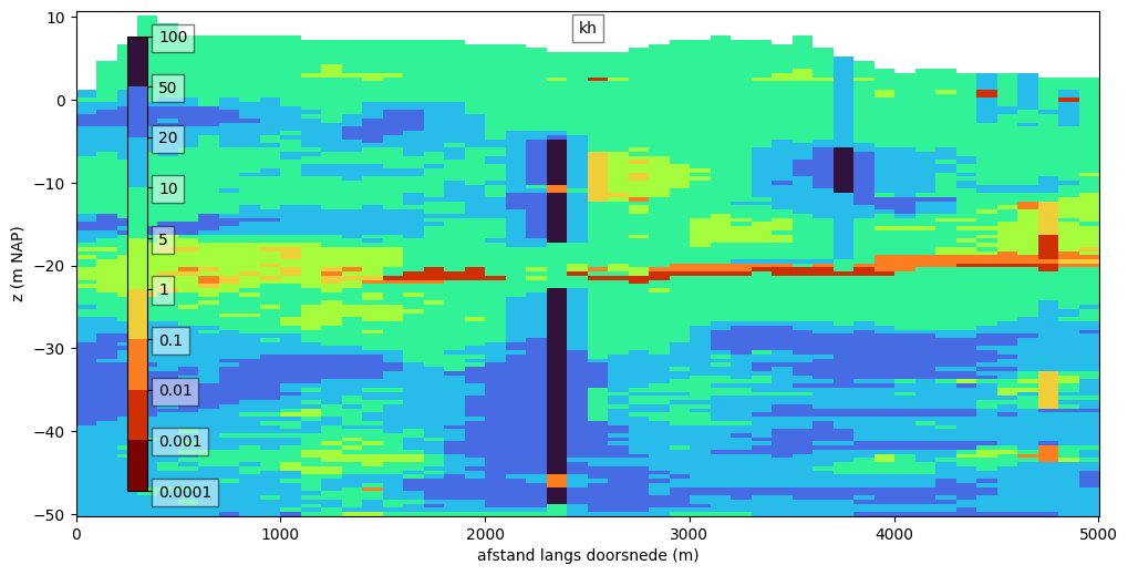
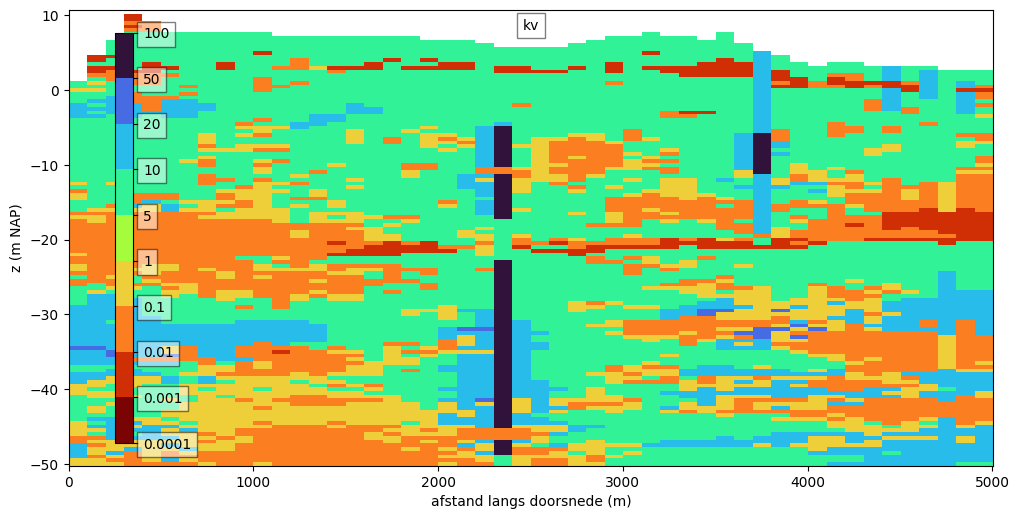
The method nlmod.read.geotop.add_kh_and_kv takes this DataFrame, applies it to the GeoTOP voxel-dataset gt, and adds the variables kh and kv to gt.
gt = nlmod.read.geotop.add_kh_and_kv(gt, df)
INFO:nlmod.read.geotop.add_kh_and_kv:Determining kh and kv of geotop-data based on lithoclass
INFO:nlmod.read.geotop.add_kh_and_kv:Setting kv equal to kh / 1.0
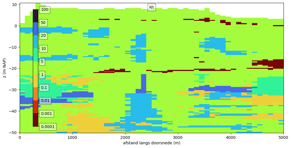
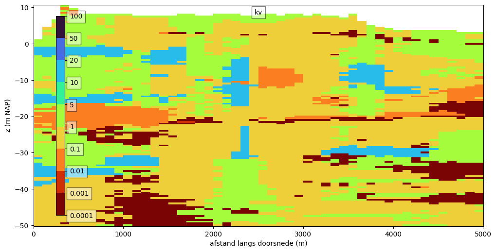
When we plot kh and kv we see fine sands get a value of 5 m/d (green) and medium fine sands get a value of 10 m/d (light blue). We see the peat (0.001 m/d) and clay (0.01 m/d) layers as zones with lower conductivities.
plot_kh_kv(gt, layer="z")

Based on lithok and strat
We can also load one of the other DataFrames that are built into nlmod, using the method nlmod.geotop.get_kh_kv_table(). Using this method, a table for certain location can be loaded. Right now, the only allowed value for kind is ‘Brabant’, which is the default value, and loads the hydrological properties per lithoclass and stratigraphic unit.
df_brab = nlmod.read.geotop.get_kh_kv_table(kind="Brabant")
df_brab
| Eenheid | strat | Beschrijving | lithok | Lithoklasse | kh | kv | |
|---|---|---|---|---|---|---|---|
| 0 | AAES | 1005 | Antropogene afzettingen, esdekken | 1 | Organisch materiaal (veen) | 0.049000 | 0.049000 |
| 1 | AAES | 1005 | Antropogene afzettingen, esdekken | 2 | Klei | 0.004000 | 0.004000 |
| 2 | AAES | 1005 | Antropogene afzettingen, esdekken | 3 | Kleiig zand, zandige klei en leem | 0.004000 | 0.004000 |
| 3 | AAES | 1005 | Antropogene afzettingen, esdekken | 5 | Fijn zand | 1.386546 | 0.566130 |
| 4 | AAES | 1005 | Antropogene afzettingen, esdekken | 6 | Midden zand | 1.688105 | 0.486891 |
| ... | ... | ... | ... | ... | ... | ... | ... |
| 392 | USER INPUT | 2000 | Formatie van Naaldwijk | 3 | Kleiig zand, zandige klei en leem | 1.636938 | 0.018171 |
| 393 | USER INPUT | 2000 | Formatie van Naaldwijk | 5 | Fijn zand | 1.129415 | 0.617087 |
| 394 | USER INPUT | 2000 | Formatie van Naaldwijk | 6 | Midden zand | 4.431265 | 2.493453 |
| 395 | USER INPUT | 2000 | Formatie van Naaldwijk | 7 | Grof zand, grind en schelpen | 14.813521 | 13.799374 |
| 396 | USER INPUT | 2000 | Formatie van Naaldwijk | 8 | Grind (indien apart gemodelleerd) | 85.100000 | 85.100000 |
397 rows × 7 columns
We use this table to add a kh and kv value for each voxel, in variables named ‘kh’ and ‘kv’.
gt_brab = nlmod.read.geotop.add_kh_and_kv(gt.copy(), df_brab)
gt_brab
INFO:nlmod.read.geotop.add_kh_and_kv:Determining kh and kv of geotop-data based on lithoclass and stratigraphy
<xarray.Dataset> Size: 2MB
Dimensions:  (z: 313, y: 2, x: 50)
Coordinates:
  * z        (z) float32 1kB 106.0 105.5 105.0 104.5 ... -48.5 -49.0 -49.5 -50.0
  * y        (y) float64 16B 5e+05 4.998e+05
  * x        (x) float64 400B 1e+05 1.002e+05 1.002e+05 ... 1.048e+05 1.05e+05
Data variables: (12/17)
    strat    (z, y, x) float32 125kB dask.array<chunksize=(9, 2, 50), meta=np.ndarray>
    lithok   (z, y, x) float32 125kB dask.array<chunksize=(9, 2, 50), meta=np.ndarray>
    kans_1   (z, y, x) float32 125kB dask.array<chunksize=(9, 2, 50), meta=np.ndarray>
    kans_2   (z, y, x) float32 125kB dask.array<chunksize=(9, 2, 50), meta=np.ndarray>
    kans_3   (z, y, x) float32 125kB dask.array<chunksize=(9, 2, 50), meta=np.ndarray>
    kans_4   (z, y, x) float32 125kB dask.array<chunksize=(9, 2, 50), meta=np.ndarray>
    ...       ...
    onz_lk   (z, y, x) float32 125kB dask.array<chunksize=(9, 2, 50), meta=np.ndarray>
    onz_ls   (z, y, x) float32 125kB dask.array<chunksize=(9, 2, 50), meta=np.ndarray>
    botm     (z, y, x) float32 125kB nan nan nan nan ... -50.25 -50.25 -50.25
    top      (z, y, x) float32 125kB nan nan nan nan ... -49.75 -49.75 -49.75
    kh       (z, y, x) float64 250kB nan nan nan nan ... 2.958 11.63 11.63 11.63
    kv       (z, y, x) float64 250kB nan nan nan nan ... 2.961 2.961 2.961
Attributes:
    title:         geotop v01r6s1 (100.0m * 100.0m * 0.5m
    references:    http://www.dinoloket.nl/detaillering-van-de-bovenste-lagen...
    comment:       GeoTOP 1.6.1 (lithoklasse)
    disclaimer:    http://www.dinoloket.nl
    terms_of_use:  http://www.dinoloket.nl
    institution:   TNO / Geologische Dienst Nederland
    Conventions:   CF-1.4
    source:        Generated by nl.tno.dino.geo3dmodel.generator.GeoTOPVoxelM...
history: Generated on Thu May 01 22:54:36 CEST 2025We can plot these values along the same line we plotted the lithoclass-values in.
plot_kh_kv(gt_brab, layer="z")
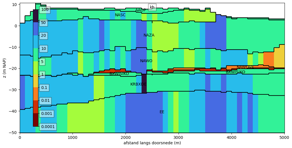
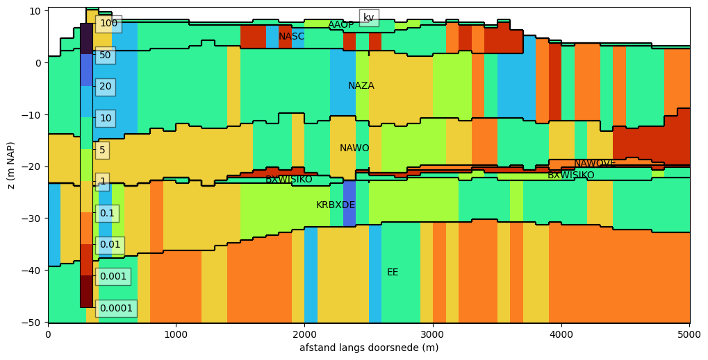
Aggregate voxels to GeoTOP-layers
In the previous example we have added geodrological properties to the voxels of GeoTOP and plotted them. The layers of a groundwatermodel generally are thicker than the thickness of the voxels (0.5 m). Therefore we need to aggregate the voxel-data into the layers of the model. We show this process by using the stratigraphy-data of GeoTOP to form a layer model, using the method nlmod.read.geotop.to_model_layers.
When values for kh and kv are present in gt, this method also calculates the geohydrological properties of the layer model with the method nlmod.read.geotop.aggregate_to_ds. The method calculates the combined horizontal transmissivity, and the combined vertical resistance of all (parts of) voxels in a layer, and calculates a kh and kv value from this transmissivity and resistance.
gtl = nlmod.read.geotop.to_model_layers(gt)
gtl
<xarray.Dataset> Size: 23kB
Dimensions:  (y: 2, x: 50, layer: 9)
Coordinates:
  * y        (y) float64 16B 5e+05 4.998e+05
  * x        (x) float64 400B 1e+05 1.002e+05 1.002e+05 ... 1.048e+05 1.05e+05
  * layer    (layer) <U8 288B 'AAOP' 'NASC' 'NAZA' ... 'BXWISIKO' 'KRBXDE' 'EE'
Data variables:
    top      (y, x) float64 800B 0.75 2.25 5.75 9.25 ... 3.75 2.75 2.75 3.25
    botm     (layer, y, x) float64 7kB 0.75 2.25 5.75 ... -50.25 -50.25 -50.25
    kh       (layer, y, x) float64 7kB nan nan nan nan ... 8.588 8.292 14.41
    kv       (layer, y, x) float64 7kB nan nan nan ... 0.04108 0.02668 0.03769
Attributes:
geulen: []We can plot the kh and kv value for each of the layers with the same method we used for the voxel-data.
plot_kh_kv(gtl, min_label_area=1000.0)
Aggregate voxels to REGIS-layers
We can use any layer model in nlmod.read.geotop.aggregate_to_ds(), also one from REGIS. Let’s demonstrate this by downloading REGIS-data for the same extent.
regis = nlmod.read.download_regis(extent)
regis
WARNING:nlmod.dims.layers.remove_layer_dim_from_top:Botm of layer is not equal to top of deeper layer in 2 cells
<xarray.Dataset> Size: 45kB
Dimensions: (y: 2, x: 50, layer: 36)
Coordinates:
* y (y) float64 16B 5e+05 4.998e+05
* x (x) float64 400B 1e+05 1.002e+05 ... 1.048e+05 1.05e+05
* layer (layer) <U8 1kB 'HLc' 'KRz3' 'EEz1' ... 'OOz2' 'OOc' 'BRk1'
spatial_ref int64 8B 0
Data variables:
top (y, x) float32 400B 0.9 2.36 6.05 9.6 ... 3.83 3.09 3.08 3.37
botm (layer, y, x) float32 14kB -25.45 -25.48 ... -816.7 -816.8
kh (layer, y, x) float32 14kB nan nan nan nan ... nan nan nan nan
kv (layer, y, x) float32 14kB nan nan nan ... 0.002 0.002 0.002
Attributes: (12/41)
references: https://www.dinoloket.nl/regis-ii-het-hydr...
Conventions: CF-1.7
creator_url: https://www.dinoloket.nl
keywords_vocabulary: NASA/GCMD Earth Science Keywords. Version 6.0
acknowledgment: https://www.dinoloket.nl
project: REGIS v02r2s3
... ...
geospatial_vertical_min: -1235.92
geospatial_vertical_max: 322.75
geospatial_vertical_units: m-NAP
geospatial_vertical_positive: up
gridtype: structured
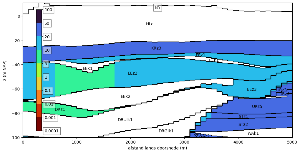
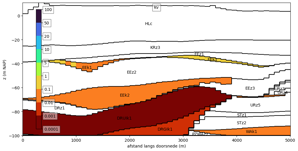
extent: [100000.0, 105000.0, 499800.0, 500000.0]First we plot the original hydrological properties of REGIS. We see that kh is defined for the aquifers (top plot) and kv is defined for the aquitards (bottom plot). Neither kh or kv is defined for the top layer HLc.
plot_kh_kv(regis, min_label_area=1000.0, zmin=-100.0)
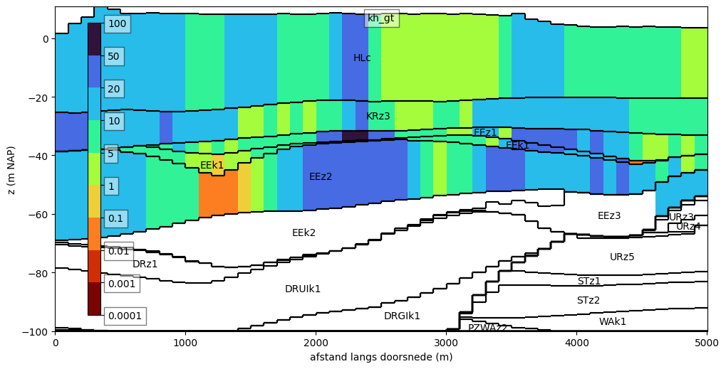
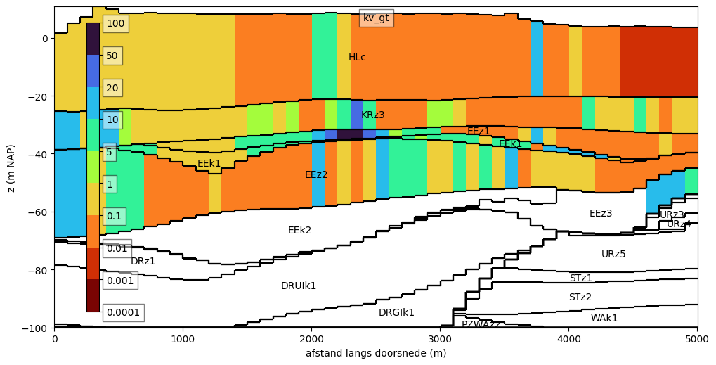
We will add varibales kh_gt and kv_gt that contain the kh- and kv-values calculated from GeoTOP. Layers that do not contain any voxel will get a NaN-value for kh and kv.
# make sure there are no NaNs in top and botm of layers
regis = nlmod.read.geotop.aggregate_to_ds(gt, regis, kh="kh_gt", kv="kv_gt")
When we plot the kh and kv value, we see all layers above -50 m NAP now contain values, calculated from the GeoTOP-data.
plot_kh_kv(regis, min_label_area=1000.0, zmin=-100.0, variables=["kh_gt", "kv_gt"])
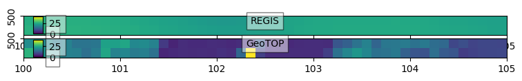
We can plot kh of one of the layers on a map, for both REGIS and GeoTOP. We generally see that conductivities in GeoTOP are a bit lower.
layer = "KRz3"
var = "kh"
norm = matplotlib.colors.Normalize(0.0, 40.0)

f, axes = nlmod.plot.get_map(extent, nrows=2)
pc = nlmod.plot.data_array(regis[var].loc[layer], ax=axes[0], norm=norm)
nlmod.plot.colorbar_inside(pc, bounds=[0.02, 0.05, 0.02, 0.9], ax=axes[0])
nlmod.plot.title_inside("REGIS", ax=axes[0])
pc = nlmod.plot.data_array(regis[f"{var}_gt"].loc[layer], ax=axes[1], norm=norm)
nlmod.plot.title_inside("GeoTOP", ax=axes[1])
nlmod.plot.colorbar_inside(pc, bounds=[0.02, 0.05, 0.02, 0.9], ax=axes[1]);
WARNING:py.warnings._showwarnmsg:/home/docs/checkouts/readthedocs.org/user_builds/nlmod/envs/latest/lib/python3.11/site-packages/IPython/core/events.py:100: UserWarning: constrained_layout not applied because axes sizes collapsed to zero.  Try making figure larger or Axes decorations smaller.
  func(*args, **kwargs)

WARNING:py.warnings._showwarnmsg:/home/docs/checkouts/readthedocs.org/user_builds/nlmod/envs/latest/lib/python3.11/site-packages/IPython/core/pylabtools.py:170: UserWarning: constrained_layout not applied because axes sizes collapsed to zero.  Try making figure larger or Axes decorations smaller.
  fig.canvas.print_figure(bytes_io, **kw)
Using stochastic data from GeoTOP
In the previous section we used the most likely values from the lithoclass data of GeoTOP. GeoTOP is constructed by generating 100 realisations of this data. Using these realisations a probablity is determined for the occurence in each pixel for each of the lithoclassses. We can also use these probabilities to determine the kh and kv-value of each voxel. We do this by settting the stochastic parameter in nlmod.read.geotop.add_kh_and_kv to True. The kh and kv values are now calculated by a weighted average of the lithoclass data in each voxel, where the weights are determined by the probablilities. By default an arithmetic weighted mean is used for kh and a harmonic weighted mean for kv, but these methods can be chosen by the user.
gt = nlmod.read.geotop.add_kh_and_kv(gt, df, stochastic=True)
INFO:nlmod.read.geotop.add_kh_and_kv:Determining kh and kv of geotop-data based on lithoclass
INFO:nlmod.read.geotop.add_kh_and_kv:Setting kv equal to kh / 1.0
We can plot the kh- and kv-values again. Using the stochastic data generally results in smoother values for kh and kv.
plot_kh_kv(gt, layer="z")
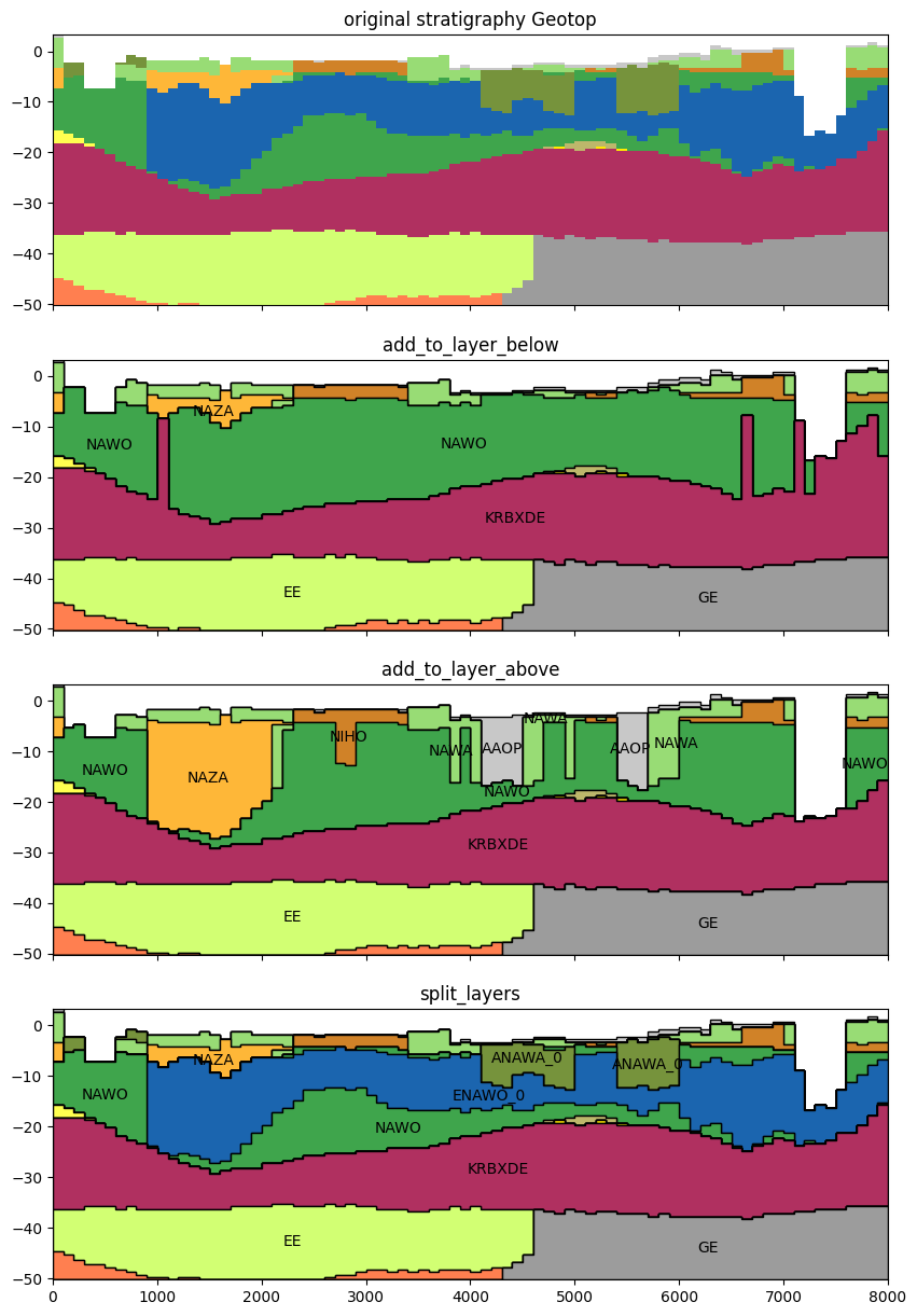
Geulen
Most of the stratigraphic units in Geotop are layered on top of each other. Meaning that these stratipgrahic units are always completely on top or completely below the other units. The so-called “geulen” are the exception to this, they can occur above, in-between and below other units. This makes it harderd to construct a layered groundwatermodel from the stratigraphic units.
Currently there are three options to create a layer model based on the stratigraphic units in geotop:
add_to_layer_below, a geul is added to the layer directly below the geuladd_to_layer_above, a geul is added to the layer directly above the geulsplit_layers, the geul is added as seperate layers in the layer model. If a geul occurs both above and below another unit this unit is also split into two layers.
Below an example to showcase the differences between these methods. For this we use a different extent with 2 geulen in the stratigraphic geotop data.
# This extent has two Geulen in it
extent = (106000.0, 114000.0, 490500.0, 490700.0)
line1 = LineString([(extent[0], extent[2]+50), (extent[1], extent[2]+50)])
line2 = LineString([(extent[0], extent[2]+150), (extent[1], extent[2]+150)])

# download geotop
gt = nlmod.read.geotop.download_geotop(extent)

# add hydrological properties
df = nlmod.read.geotop.get_lithok_props()
gt = nlmod.read.geotop.add_kh_and_kv(gt, df)

# set the logger to debug to get all the information
logger = nlmod.util.get_color_logger("DEBUG")
gtl1 = nlmod.read.geotop.to_model_layers(gt, method_geulen='add_to_layer_below')
gtl2 = nlmod.read.geotop.to_model_layers(gt, method_geulen='add_to_layer_above')
gtl3 = nlmod.read.geotop.to_model_layers(gt, method_geulen='split_layers')
INFO:nlmod.read.geotop.add_kh_and_kv:Determining kh and kv of geotop-data based on lithoclass
INFO:nlmod.read.geotop.add_kh_and_kv:Setting kv equal to kh / 1.0
WARNING:nlmod.dims.layers.remove_layer_dim_from_top:1350:Botm of layer is not equal to top of deeper layer in 27 cells
WARNING:nlmod.read.geotop.to_model_layers:522:Geul ANAWA is at the top of the GeoTOP-dataset in 9 cells, where it is ignored
WARNING:nlmod.read.geotop.to_model_layers:522:Geul ENAWO is at the top of the GeoTOP-dataset in 13 cells, where it is ignored
WARNING:nlmod.read.geotop.to_model_layers:408:the 'split_layers' method for geulen is still experimental and not yet thoroughly tested.
DEBUG:nlmod.read.geotop.split_layers_on_geul:307:geul 6010 below and above unit 1100
DEBUG:nlmod.read.geotop.split_layers_on_geul:309:split 1100, part above geul is 11100
DEBUG:nlmod.read.geotop.split_layers_on_geul:315:adding geul 6010 below unit 11100 as 26010
DEBUG:nlmod.read.geotop.split_layers_on_geul:330:adding geul 6010 below unit 1040 as 36010
DEBUG:nlmod.read.geotop.split_layers_on_geul:330:adding geul 6010 below unit 1000 as 46010
DEBUG:nlmod.read.geotop.split_layers_on_geul:339:new order of units: [np.int64(1000), np.int64(46010), np.int64(1030), np.int64(1040), np.int64(36010), np.int64(1050), np.int64(1090), np.int64(11100), np.int64(26010), np.int64(1100), np.int64(1120), np.int64(1130), np.int64(3030), np.int64(3100), np.int64(4010), np.int64(4110), np.int64(5000), np.int64(5020)]
DEBUG:nlmod.read.geotop.split_layers_on_geul:307:geul 6420 below and above unit 1100
DEBUG:nlmod.read.geotop.split_layers_on_geul:309:split 1100, part above geul is 21100
DEBUG:nlmod.read.geotop.split_layers_on_geul:315:adding geul 6420 below unit 21100 as 26420
DEBUG:nlmod.read.geotop.split_layers_on_geul:339:new order of units: [np.int64(1000), np.int64(46010), np.int64(1030), np.int64(1040), np.int64(36010), np.int64(1050), np.int64(1090), np.int64(11100), np.int64(26010), np.int64(21100), np.int64(26420), np.int64(1100), np.int64(1120), np.int64(1130), np.int64(3030), np.int64(3100), np.int64(4010), np.int64(4110), np.int64(5000), np.int64(5020)]
# plot layer models
logger = nlmod.util.get_color_logger("INFO")
stratdf = nlmod.read.geotop.get_strat_props().set_index('code')
f, axes = plt.subplots(figsize=(10, 15), nrows=4, sharex=True)

nlmod.plot.geotop_strat_in_cross_section(line1, gt, ax=axes[0], legend=False)
axes[0].set_title('original stratigraphy Geotop')

cs1 = nlmod.plot.DatasetCrossSection(gtl1, line1, layer='layer', ax=axes[1])
out1 = cs1.plot_layers(colors=stratdf, edgecolor='k',  min_label_area=3000)
axes[1].set_title('add_to_layer_below')

cs2 = nlmod.plot.DatasetCrossSection(gtl2, line1, layer='layer', ax=axes[2])
out2 = cs2.plot_layers(colors=stratdf, edgecolor='k',  min_label_area=3000)
axes[2].set_title('add_to_layer_above')

cs3 = nlmod.plot.DatasetCrossSection(gtl3, line1, layer='layer', ax=axes[3])
out3 = cs3.plot_layers(colors=stratdf, edgecolor='k', min_label_area=3000)
axes[3].set_title('split_layers');

print('units in original gt:', sum(~np.isnan(np.unique(gt['strat']))))
print('layers in gtl1:', len(gtl1.layer))
print('layers in gtl2:', len(gtl2.layer))
print('layers in gtl3:', len(gtl3.layer))
units in original gt: 16
layers in gtl1: 14
layers in gtl2: 14
layers in gtl3: 20