A groundwater model for Schoonhoven

In this notebook we build a transient model for the area around Schoonhoven. Surface water is added to the model using a winter and a summer stage using the drain package. For the river Lek, we build a river package with a fixed stage of NAP+0.0 m.

import os

import flopy
import geopandas as gpd
import matplotlib
import matplotlib.pyplot as plt
import numpy as np
import pandas as pd
from shapely.geometry import LineString, Point

import nlmod
from nlmod.plot import DatasetCrossSection

nlmod.util.get_color_logger("INFO")
nlmod.show_versions()

Python version     : 3.11.14
NumPy version      : 2.4.4
Xarray version     : 2026.4.0
Matplotlib version : 3.10.9
Flopy version      : 3.10.0

nlmod version      : 0.11.3dev

Model settings

We define some model settings, like the name, the directory of the model files, the model extent and the time

model_name = "Schoonhoven"
model_ws = "09_schoonhoven"
figdir, cachedir = nlmod.util.get_model_dirs(model_ws)
extent = [116_500, 120_000, 439_000, 442_000]
time = pd.date_range("2020", "2023", freq="MS")  # monthly timestep

Download data

layer ‘waterdeel’ from bgt

The location of the surface water bodies is obtained from the GeoDataFrame that was created in the the surface water notebook. We saved this data as a geosjon file and load it here.

fname_bgt = os.path.join("..", "data_sources", "02_surface_water", "cache", "bgt.gpkg")
if not os.path.isfile(fname_bgt):
    raise (
        Exception(
            f"{fname_bgt} not found. Please run notebook 02_surface_water.ipynb in the 'data_sources' directory first"
        )
    )
bgt = gpd.read_file(fname_bgt)

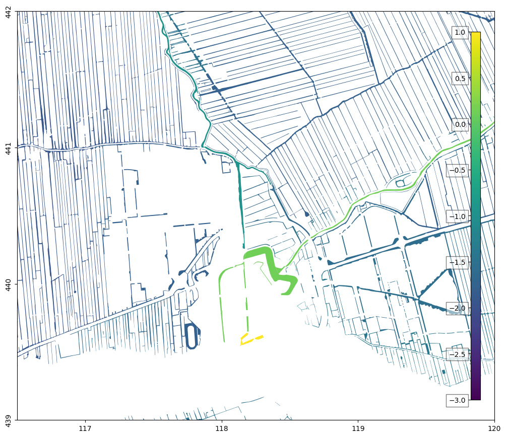
Plot summer stage of surface water bodies

We can plot the summer stage. There are some surface water bodies without a summer stage, because the ‘bronhouder’ is not a water board. The main one is the river Lek, but there are also some surface water bodies without a summer stage in the north of the model area.

f, ax = nlmod.plot.get_map(extent)
norm = matplotlib.colors.Normalize(vmin=-3, vmax=1)
cmap = "viridis"
bgt.plot("summer_stage", ax=ax, norm=norm, cmap=cmap)
nlmod.plot.colorbar_inside(norm=norm, cmap=cmap);

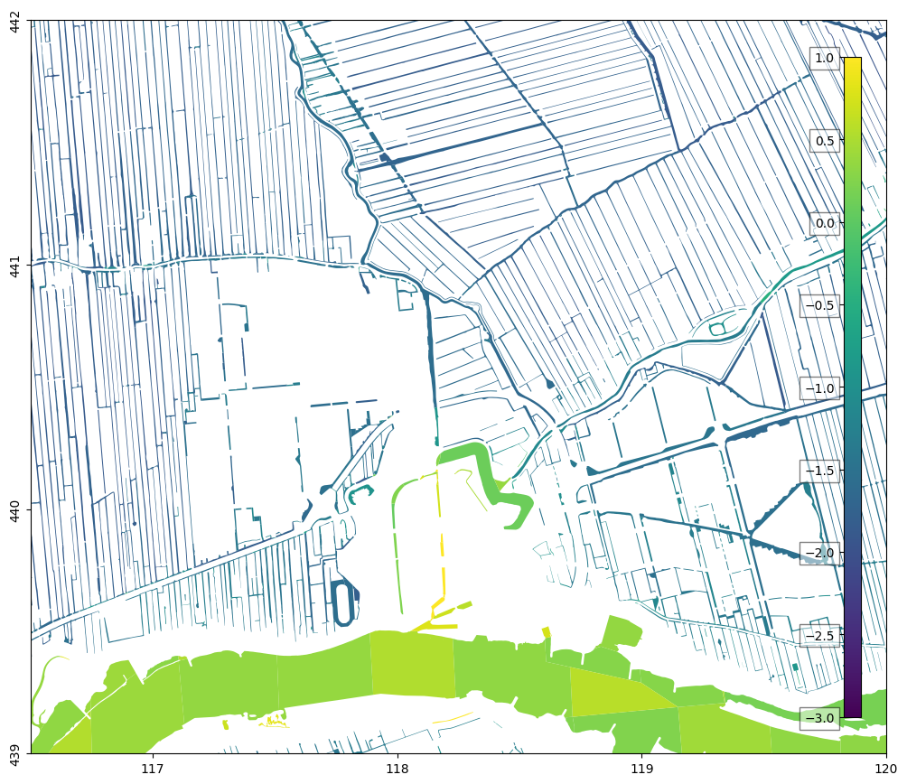
If no information about the stage is available, a constant stage is set to the minimal height of the digital terrain model (AHN) near the surface water body. We can plot these values as well:

f, ax = nlmod.plot.get_map(extent)
bgt.plot("ahn_min", ax=ax, norm=norm, cmap=cmap)
nlmod.plot.colorbar_inside(norm=norm, cmap=cmap);

KNMI

KNMI precipitation and evaporation data is used to estimate the recharge.

# knmi data
oc_knmi = nlmod.read.knmi.download_knmi(extent=extent, delr=100., delc=100., start='2000-1-1', end='2025-1-1')

INFO:nlmod.dims.base.to_model_ds:resample layer model data to structured modelgrid
INFO:hydropandas.io.knmi.get_knmi_obs:get data from station 434 and variable RD from 2000-01-01 to 2025-01-01
INFO:hydropandas.io.knmi.get_knmi_obs:get data from station 348 and variable EV24 from 2000-01-01 to 2025-01-01

REGIS

For the schematisation of the subsurface we use REGIS. Let’s download this data for the required extent.

layer_model = nlmod.read.regis.get_combined_layer_models(
    extent,
    use_regis=True,
    use_geotop=False,
    cachedir=cachedir,
    cachename="layer_model.nc",
)
layer_model

WARNING:nlmod.dims.layers.remove_layer_dim_from_top:Botm of layer is not equal to top of deeper layer in 3 cells
INFO:nlmod.cache.wrapper:caching data -> layer_model.nc

<xarray.Dataset> Size: 371kB
Dimensions:      (y: 30, x: 35, layer: 29)
Coordinates:
  * y            (y) float64 240B 4.42e+05 4.418e+05 ... 4.392e+05 4.39e+05
  * x            (x) float64 280B 1.166e+05 1.166e+05 ... 1.198e+05 1.2e+05
  * layer        (layer) <U8 928B 'HLc' 'KRWYk1' 'KRz2' ... 'OOz2' 'OOc' 'BRk1'
    spatial_ref  int64 8B 0
Data variables:
    top          (y, x) float32 4kB -1.28 -1.22 -1.25 ... -4.05 -3.76 -4.21
    botm         (layer, y, x) float32 122kB -12.26 -12.11 ... -593.9 -595.5
    kh           (layer, y, x) float32 122kB nan nan nan nan ... nan nan nan nan
    kv           (layer, y, x) float32 122kB nan nan nan ... 0.002 0.002 0.002
Attributes: (12/41)
    references:                    https://www.dinoloket.nl/regis-ii-het-hydr...
    Conventions:                   CF-1.7
    creator_url:                   https://www.dinoloket.nl
    keywords_vocabulary:           NASA/GCMD Earth Science Keywords. Version 6.0
    acknowledgment:                https://www.dinoloket.nl
    project:                       REGIS v02r2s3
    ...                            ...
    geospatial_vertical_min:       -1235.92
    geospatial_vertical_max:       322.75
    geospatial_vertical_units:     m-NAP
    geospatial_vertical_positive:  up
    gridtype:                      structured
    extent:                        [116500, 120000, 439000, 442000]

xarray.Dataset

• Dimensions:
  • y: 30
  • x: 35
  • layer: 29
• Coordinates: (4)
  • y
    (y)
    float64
    4.42e+05 4.418e+05 ... 4.39e+05

    comment :

    y-coordinate values at the upper and lower bounds of each pixel.

    array([441950., 441850., 441750., 441650., 441550., 441450., 441350., 441250.,
           441150., 441050., 440950., 440850., 440750., 440650., 440550., 440450.,
           440350., 440250., 440150., 440050., 439950., 439850., 439750., 439650.,
           439550., 439450., 439350., 439250., 439150., 439050.])

  • x
    (x)
    float64
    1.166e+05 1.166e+05 ... 1.2e+05

    comment :

    x-coordinate values at the left and right bounds of each pixel.

    array([116550., 116650., 116750., 116850., 116950., 117050., 117150., 117250.,
           117350., 117450., 117550., 117650., 117750., 117850., 117950., 118050.,
           118150., 118250., 118350., 118450., 118550., 118650., 118750., 118850.,
           118950., 119050., 119150., 119250., 119350., 119450., 119550., 119650.,
           119750., 119850., 119950.])

  • layer
    (layer)
    <U8
    'HLc' 'KRWYk1' ... 'OOc' 'BRk1'

    array(['HLc', 'KRWYk1', 'KRz2', 'KRz3', 'URz1', 'URz3', 'URz4', 'URz5', 'STz1',
           'STz2', 'SYk1', 'PZWAz1', 'WAk1', 'PZWAz2', 'WAk2', 'PZWAz3', 'WAk3',
           'PZWAz4', 'MSz1', 'MSk1', 'MSz2', 'MSk2', 'MSz3', 'MSc', 'MSz4', 'OOk1',
           'OOz2', 'OOc', 'BRk1'], dtype='<U8')

  • spatial_ref
    ()
    int64
    0

    crs_wkt :

    PROJCS["Amersfoort / RD New",GEOGCS["Amersfoort",DATUM["Amersfoort",SPHEROID["Bessel 1841",6377397.155,299.1528128,AUTHORITY["EPSG","7004"]],AUTHORITY["EPSG","6289"]],PRIMEM["Greenwich",0,AUTHORITY["EPSG","8901"]],UNIT["degree",0.0174532925199433,AUTHORITY["EPSG","9122"]],AUTHORITY["EPSG","4289"]],PROJECTION["Oblique_Stereographic"],PARAMETER["latitude_of_origin",52.1561605555556],PARAMETER["central_meridian",5.38763888888889],PARAMETER["scale_factor",0.9999079],PARAMETER["false_easting",155000],PARAMETER["false_northing",463000],UNIT["metre",1,AUTHORITY["EPSG","9001"]],AXIS["Easting",EAST],AXIS["Northing",NORTH],AUTHORITY["EPSG","28992"]]

    spatial_ref :

    PROJCS["Amersfoort / RD New",GEOGCS["Amersfoort",DATUM["Amersfoort",SPHEROID["Bessel 1841",6377397.155,299.1528128,AUTHORITY["EPSG","7004"]],AUTHORITY["EPSG","6289"]],PRIMEM["Greenwich",0,AUTHORITY["EPSG","8901"]],UNIT["degree",0.0174532925199433,AUTHORITY["EPSG","9122"]],AUTHORITY["EPSG","4289"]],PROJECTION["Oblique_Stereographic"],PARAMETER["latitude_of_origin",52.1561605555556],PARAMETER["central_meridian",5.38763888888889],PARAMETER["scale_factor",0.9999079],PARAMETER["false_easting",155000],PARAMETER["false_northing",463000],UNIT["metre",1,AUTHORITY["EPSG","9001"]],AXIS["Easting",EAST],AXIS["Northing",NORTH],AUTHORITY["EPSG","28992"]]

    array(0)

• Data variables: (4)
  • top
    (y, x)
    float32
    -1.28 -1.22 -1.25 ... -3.76 -4.21

    long_name :

    top

    standard_name :

    depth_of_top_of_layer

    units :

    mNAP

    source :

    REGIS

    url :

    https://www.dinodata.nl/opendap/REGIS/REGIS.nc

    date :

    20260513

    array([[-1.28, -1.22, -1.25, ..., -1.24, -1.33, -1.26],
           [-1.26, -1.17, -1.24, ..., -1.11, -1.16, -1.3 ],
           [-1.29, -1.17, -1.27, ..., -1.  , -1.22, -1.3 ],
           ...,
           [ 1.17,  1.17, -0.1 , ..., -0.05,  0.15, -0.57],
           [ 0.69, -1.59, -3.38, ...,  1.18, -0.63, -0.66],
           [-0.91, -3.74, -5.36, ..., -4.05, -3.76, -4.21]],
          shape=(30, 35), dtype=float32)

  • botm
    (layer, y, x)
    float32
    -12.26 -12.11 ... -593.9 -595.5

    long_name :

    bottom

    standard_name :

    depth_of_bottom_of_layer

    units :

    mNAP

    source :

    REGIS

    url :

    https://www.dinodata.nl/opendap/REGIS/REGIS.nc

    date :

    20260513

    array([[[ -12.26,  -12.11,  -11.93, ...,  -10.96,  -10.87,  -10.84],
            [ -12.34,  -12.18,  -11.98, ...,  -10.89,  -10.87,  -10.84],
            [ -12.41,  -12.25,  -12.05, ...,  -10.9 ,  -10.87,  -10.84],
            ...,
            [ -12.92,  -12.86,  -12.74, ...,  -11.09,  -11.06,  -11.07],
            [ -12.89,  -12.83,  -12.76, ...,  -11.1 ,  -11.07,  -11.08],
            [ -12.85,  -12.8 ,  -12.74, ...,  -11.11,  -11.12,  -11.09]],
    
           [[ -12.26,  -12.11,  -11.93, ...,  -11.17,  -11.18,  -11.19],
            [ -12.34,  -12.18,  -11.98, ...,  -11.14,  -11.15,  -11.16],
            [ -12.41,  -12.25,  -12.05, ...,  -11.1 ,  -11.11,  -11.12],
            ...,
            [ -12.92,  -12.86,  -12.74, ...,  -11.09,  -11.06,  -11.07],
            [ -12.89,  -12.83,  -12.76, ...,  -11.1 ,  -11.07,  -11.08],
            [ -12.85,  -12.8 ,  -12.74, ...,  -11.11,  -11.12,  -11.09]],
    
           [[ -13.17,  -13.03,  -12.87, ...,  -12.06,  -11.97,  -11.94],
            [ -13.28,  -13.12,  -12.94, ...,  -12.03,  -12.  ,  -11.97],
            [ -13.37,  -13.21,  -13.02, ...,  -12.07,  -12.03,  -12.  ],
            ...,
    ...
            [-326.14, -326.17, -326.2 , ..., -325.79, -325.75, -325.71],
            [-326.19, -326.1 , -326.13, ..., -325.75, -325.71, -325.67],
            [-326.12, -326.15, -326.17, ..., -325.71, -325.67, -325.62]],
    
           [[-368.87, -368.48, -368.  , ..., -363.1 , -363.09, -363.06],
            [-368.44, -367.94, -367.44, ..., -362.64, -362.64, -362.64],
            [-368.1 , -367.41, -366.89, ..., -362.21, -362.23, -362.23],
            ...,
            [-365.17, -364.72, -364.16, ..., -359.84, -359.92, -359.97],
            [-365.63, -365.07, -364.58, ..., -360.09, -360.12, -360.15],
            [-365.99, -365.36, -364.97, ..., -360.37, -360.39, -360.4 ]],
    
           [[-502.26, -503.93, -505.66, ..., -551.66, -553.08, -554.67],
            [-502.73, -504.44, -506.24, ..., -553.3 , -554.7 , -556.21],
            [-503.26, -505.03, -506.88, ..., -554.88, -556.22, -557.84],
            ...,
            [-532.1 , -533.2 , -534.37, ..., -593.62, -594.94, -595.81],
            [-532.73, -533.75, -534.87, ..., -593.  , -594.45, -595.98],
            [-533.32, -534.27, -535.31, ..., -592.32, -593.89, -595.55]]],
          shape=(29, 30, 35), dtype=float32)

  • kh
    (layer, y, x)
    float32
    nan nan nan nan ... nan nan nan nan

    long_name :

    kh

    standard_name :

    horizontale_doorlatendheid_(kh)

    units :

    m/day

    source :

    REGIS

    url :

    https://www.dinodata.nl/opendap/REGIS/REGIS.nc

    date :

    20260513

    array([[[  nan,   nan,   nan, ...,   nan,   nan,   nan],
            [  nan,   nan,   nan, ...,   nan,   nan,   nan],
            [  nan,   nan,   nan, ...,   nan,   nan,   nan],
            ...,
            [  nan,   nan,   nan, ...,   nan,   nan,   nan],
            [  nan,   nan,   nan, ...,   nan,   nan,   nan],
            [  nan,   nan,   nan, ...,   nan,   nan,   nan]],
    
           [[  nan,   nan,   nan, ...,   nan,   nan,   nan],
            [  nan,   nan,   nan, ...,   nan,   nan,   nan],
            [  nan,   nan,   nan, ...,   nan,   nan,   nan],
            ...,
            [  nan,   nan,   nan, ...,   nan,   nan,   nan],
            [  nan,   nan,   nan, ...,   nan,   nan,   nan],
            [  nan,   nan,   nan, ...,   nan,   nan,   nan]],
    
           [[56.61, 57.18, 57.66, ..., 38.27, 37.81, 37.36],
            [55.45, 56.04, 56.51, ..., 37.59, 37.05, 36.65],
            [54.2 , 54.8 , 55.33, ..., 36.9 , 36.88, 36.04],
            ...,
    ...
            [ 7.86,  7.84,  7.82, ...,  7.47,  7.48,  7.48],
            [ 7.86,  7.84,  7.73, ...,  7.46,  7.45,  7.45],
            [ 7.88,  7.83,  7.72, ...,  7.43,  7.42,  7.42]],
    
           [[ 1.21,  1.21,  1.21, ...,  1.25,  1.25,  1.26],
            [ 1.21,  1.21,  1.21, ...,  1.26,  1.26,  1.27],
            [ 1.22,  1.21,  1.21, ...,  1.27,  1.26,  1.28],
            ...,
            [ 1.34,  1.34,  1.34, ...,  1.43,  1.43,  1.44],
            [ 1.35,  1.36,  1.35, ...,  1.42,  1.43,  1.43],
            [ 1.37,  1.37,  1.37, ...,  1.41,  1.42,  1.43]],
    
           [[  nan,   nan,   nan, ...,   nan,   nan,   nan],
            [  nan,   nan,   nan, ...,   nan,   nan,   nan],
            [  nan,   nan,   nan, ...,   nan,   nan,   nan],
            ...,
            [  nan,   nan,   nan, ...,   nan,   nan,   nan],
            [  nan,   nan,   nan, ...,   nan,   nan,   nan],
            [  nan,   nan,   nan, ...,   nan,   nan,   nan]]],
          shape=(29, 30, 35), dtype=float32)

  • kv
    (layer, y, x)
    float32
    nan nan nan ... 0.002 0.002 0.002

    long_name :

    kv

    standard_name :

    verticale_doorlatendheid_(kv)

    units :

    m/day

    source :

    REGIS

    url :

    https://www.dinodata.nl/opendap/REGIS/REGIS.nc

    date :

    20260513

    array([[[       nan,        nan,        nan, ...,        nan,
                    nan,        nan],
            [       nan,        nan,        nan, ...,        nan,
                    nan,        nan],
            [       nan,        nan,        nan, ...,        nan,
                    nan,        nan],
            ...,
            [       nan,        nan,        nan, ...,        nan,
                    nan,        nan],
            [       nan,        nan,        nan, ...,        nan,
                    nan,        nan],
            [       nan,        nan,        nan, ...,        nan,
                    nan,        nan]],
    
           [[       nan,        nan,        nan, ..., 0.01483528,
             0.01504688, 0.01521849],
            [       nan,        nan,        nan, ..., 0.01478147,
             0.01492398, 0.01504013],
            [       nan,        nan,        nan, ..., 0.01469031,
             0.01487229, 0.01486955],
    ...
            [0.0071571 , 0.00716144, 0.00716829, ..., 0.00776395,
             0.00780907, 0.00788237],
            [0.00720632, 0.00721143, 0.0072237 , ..., 0.00784941,
             0.00793054, 0.00801546],
            [0.00724916, 0.00725398, 0.00726712, ..., 0.00794574,
             0.00802989, 0.00812249]],
    
           [[0.002     , 0.002     , 0.002     , ..., 0.002     ,
             0.002     , 0.002     ],
            [0.002     , 0.002     , 0.002     , ..., 0.002     ,
             0.002     , 0.002     ],
            [0.002     , 0.002     , 0.002     , ..., 0.002     ,
             0.002     , 0.002     ],
            ...,
            [0.002     , 0.002     , 0.002     , ..., 0.002     ,
             0.002     , 0.002     ],
            [0.002     , 0.002     , 0.002     , ..., 0.002     ,
             0.002     , 0.002     ],
            [0.002     , 0.002     , 0.002     , ..., 0.002     ,
             0.002     , 0.002     ]]], shape=(29, 30, 35), dtype=float32)

• Attributes: (41)

  references :

  https://www.dinoloket.nl/regis-ii-het-hydrogeologische-model

  Conventions :

  CF-1.7

  creator_url :

  https://www.dinoloket.nl

  keywords_vocabulary :

  NASA/GCMD Earth Science Keywords. Version 6.0

  acknowledgment :

  https://www.dinoloket.nl

  project :

  REGIS v02r2s3

  creator_name :

  Geological Survey of the Netherlands, part of TNO

  cdm_data_type :

  grid

  featureType :

  grid

  summary :

  The Digital Geological Model DGM is used as the basis for the regional hydrogeological model REGIS II, serving as the starting point for further subdivision of the modelled geological units into hydrogeological units, aquifers and aquitards. Using the lithological information from boreholes and additional hydrological data such as hydraulic heads and pumping tests, the hydrogeological units are characterised in terms of their hydraulic conductivity, transmissivity and vertical resistivity, vertical flow resistance. To ensure consistency between the geological and hydrogeological models, the hydrogeological units are constrained within the units of DGM. The depths to the top and the base, and the thickness of the units have been mapped in grid files at 100 x 100 metres resolution.

  license :

  cc-by-

  publisher_name :

  TNO

  creator_email :

  info@dinoloket.nl

  keywords :

  lithological classes, tops and bottoms of layers, transmissivity

  institution :

  TNO

  history :

  www.dinoloket.nl

  naming_authority :

  dinoloket.nl

  source :

  www.dinoloket.nl

  publisher_url :

  www.dinoloket.nl

  publisher_email :

  info@dinoloket.nl

  Metadata_Conventions :

  Unidata Dataset Discovery v1.0

  standard_name_vocabulary :

  CF-1.6

  title :

  REGIS v02r2s3

  id :

  7fd8576c-b6c0-4b13-a743-7a0c47df4b29

  date_created :

  2024-12-19T20:44:07Z

  date_modified :

  2024-12-19T20:44:07Z

  date_issued :

  2024-12-19T20:44:07Z

  geospatial_lat_min :

  50.669197

  geospatial_lat_max :

  53.638645

  geospatial_lat_units :

  degrees_north

  geospatial_lat_resolution :

  0.0008998327

  geospatial_lon_min :

  3.1946514

  geospatial_lon_max :

  7.428299

  geospatial_lon_units :

  degrees_east

  geospatial_lon_resolution :

  0.0014598784

  geospatial_vertical_min :

  -1235.92

  geospatial_vertical_max :

  322.75

  geospatial_vertical_units :

  m-NAP

  geospatial_vertical_positive :

  up

  gridtype :

  structured

  extent :

  [116500, 120000, 439000, 442000]

We then create a regular grid, add necessary variables and fill NaN’s. For example, REGIS does not contain information about the hydraulic conductivity of the first layer (‘HLc’). These NaN’s are replaced by a default hydraulic conductivity (kh) of 1 m/d. This probably is not a good representation of the conductivity, but at least the model will run.

ds = nlmod.to_model_ds(layer_model, model_name, model_ws, delr=100.0, delc=100.0)
ds

INFO:nlmod.dims.base.to_model_ds:resample layer model data to structured modelgrid
INFO:nlmod.dims.layers.get_kh_kv:kv and kh both undefined in layer HLc
INFO:nlmod.dims.layers._fill_var:Filling 7594 values in active cells of kh by multipying kv with an anisotropy of 10
INFO:nlmod.dims.layers._fill_var:Filling 16762 values in active cells of kv by dividing kh by an anisotropy of 10
INFO:nlmod.dims.layers._fill_var:Filling 1050 values in active cells of kh with a value of 1.0 m/day
INFO:nlmod.dims.layers._fill_var:Filling 1050 values in active cells of kv with a value of 0.1 m/day

<xarray.Dataset> Size: 379kB
Dimensions:      (y: 30, x: 35, layer: 29)
Coordinates:
  * y            (y) float64 240B 4.42e+05 4.418e+05 ... 4.392e+05 4.39e+05
  * x            (x) float64 280B 1.166e+05 1.166e+05 ... 1.198e+05 1.2e+05
  * layer        (layer) <U8 928B 'HLc' 'KRWYk1' 'KRz2' ... 'OOz2' 'OOc' 'BRk1'
    spatial_ref  int64 8B 0
Data variables:
    top          (y, x) float32 4kB -1.28 -1.22 -1.25 ... -4.05 -3.76 -4.21
    botm         (layer, y, x) float32 122kB -12.26 -12.11 ... -593.9 -595.5
    kh           (layer, y, x) float32 122kB 1.0 1.0 1.0 1.0 ... 0.02 0.02 0.02
    kv           (layer, y, x) float32 122kB 0.1 0.1 0.1 ... 0.002 0.002 0.002
    area         (y, x) float64 8kB 1e+04 1e+04 1e+04 ... 1e+04 1e+04 1e+04
Attributes:
    extent:      [116500, 120000, 439000, 442000]
    gridtype:    structured
    model_name:  Schoonhoven
    mfversion:   mf6
    created_on:  20260513_15:12:47
    exe_name:    /home/docs/checkouts/readthedocs.org/user_builds/nlmod/envs/...
    model_ws:    09_schoonhoven
    figdir:      09_schoonhoven/figure
    cachedir:    09_schoonhoven/cache
    transport:   0

xarray.Dataset

• Dimensions:
  • y: 30
  • x: 35
  • layer: 29
• Coordinates: (4)
  • y
    (y)
    float64
    4.42e+05 4.418e+05 ... 4.39e+05

    comment :

    y-coordinate values at the upper and lower bounds of each pixel.

    array([441950., 441850., 441750., 441650., 441550., 441450., 441350., 441250.,
           441150., 441050., 440950., 440850., 440750., 440650., 440550., 440450.,
           440350., 440250., 440150., 440050., 439950., 439850., 439750., 439650.,
           439550., 439450., 439350., 439250., 439150., 439050.])

  • x
    (x)
    float64
    1.166e+05 1.166e+05 ... 1.2e+05

    comment :

    x-coordinate values at the left and right bounds of each pixel.

    array([116550., 116650., 116750., 116850., 116950., 117050., 117150., 117250.,
           117350., 117450., 117550., 117650., 117750., 117850., 117950., 118050.,
           118150., 118250., 118350., 118450., 118550., 118650., 118750., 118850.,
           118950., 119050., 119150., 119250., 119350., 119450., 119550., 119650.,
           119750., 119850., 119950.])

  • layer
    (layer)
    <U8
    'HLc' 'KRWYk1' ... 'OOc' 'BRk1'

    array(['HLc', 'KRWYk1', 'KRz2', 'KRz3', 'URz1', 'URz3', 'URz4', 'URz5', 'STz1',
           'STz2', 'SYk1', 'PZWAz1', 'WAk1', 'PZWAz2', 'WAk2', 'PZWAz3', 'WAk3',
           'PZWAz4', 'MSz1', 'MSk1', 'MSz2', 'MSk2', 'MSz3', 'MSc', 'MSz4', 'OOk1',
           'OOz2', 'OOc', 'BRk1'], dtype='<U8')

  • spatial_ref
    ()
    int64
    0

    crs_wkt :

    PROJCS["Amersfoort / RD New",GEOGCS["Amersfoort",DATUM["Amersfoort",SPHEROID["Bessel 1841",6377397.155,299.1528128,AUTHORITY["EPSG","7004"]],AUTHORITY["EPSG","6289"]],PRIMEM["Greenwich",0,AUTHORITY["EPSG","8901"]],UNIT["degree",0.0174532925199433,AUTHORITY["EPSG","9122"]],AUTHORITY["EPSG","4289"]],PROJECTION["Oblique_Stereographic"],PARAMETER["latitude_of_origin",52.1561605555556],PARAMETER["central_meridian",5.38763888888889],PARAMETER["scale_factor",0.9999079],PARAMETER["false_easting",155000],PARAMETER["false_northing",463000],UNIT["metre",1,AUTHORITY["EPSG","9001"]],AXIS["Easting",EAST],AXIS["Northing",NORTH],AUTHORITY["EPSG","28992"]]

    spatial_ref :

    PROJCS["Amersfoort / RD New",GEOGCS["Amersfoort",DATUM["Amersfoort",SPHEROID["Bessel 1841",6377397.155,299.1528128,AUTHORITY["EPSG","7004"]],AUTHORITY["EPSG","6289"]],PRIMEM["Greenwich",0,AUTHORITY["EPSG","8901"]],UNIT["degree",0.0174532925199433,AUTHORITY["EPSG","9122"]],AUTHORITY["EPSG","4289"]],PROJECTION["Oblique_Stereographic"],PARAMETER["latitude_of_origin",52.1561605555556],PARAMETER["central_meridian",5.38763888888889],PARAMETER["scale_factor",0.9999079],PARAMETER["false_easting",155000],PARAMETER["false_northing",463000],UNIT["metre",1,AUTHORITY["EPSG","9001"]],AXIS["Easting",EAST],AXIS["Northing",NORTH],AUTHORITY["EPSG","28992"]]

    array(0)

• Data variables: (5)
  • top
    (y, x)
    float32
    -1.28 -1.22 -1.25 ... -3.76 -4.21

    long_name :

    top

    standard_name :

    depth_of_top_of_layer

    units :

    mNAP

    source :

    REGIS

    url :

    https://www.dinodata.nl/opendap/REGIS/REGIS.nc

    date :

    20260513

    array([[-1.28, -1.22, -1.25, ..., -1.24, -1.33, -1.26],
           [-1.26, -1.17, -1.24, ..., -1.11, -1.16, -1.3 ],
           [-1.29, -1.17, -1.27, ..., -1.  , -1.22, -1.3 ],
           ...,
           [ 1.17,  1.17, -0.1 , ..., -0.05,  0.15, -0.57],
           [ 0.69, -1.59, -3.38, ...,  1.18, -0.63, -0.66],
           [-0.91, -3.74, -5.36, ..., -4.05, -3.76, -4.21]],
          shape=(30, 35), dtype=float32)

  • botm
    (layer, y, x)
    float32
    -12.26 -12.11 ... -593.9 -595.5

    long_name :

    bottom

    standard_name :

    depth_of_bottom_of_layer

    units :

    mNAP

    source :

    REGIS

    url :

    https://www.dinodata.nl/opendap/REGIS/REGIS.nc

    date :

    20260513

    array([[[ -12.26,  -12.11,  -11.93, ...,  -10.96,  -10.87,  -10.84],
            [ -12.34,  -12.18,  -11.98, ...,  -10.89,  -10.87,  -10.84],
            [ -12.41,  -12.25,  -12.05, ...,  -10.9 ,  -10.87,  -10.84],
            ...,
            [ -12.92,  -12.86,  -12.74, ...,  -11.09,  -11.06,  -11.07],
            [ -12.89,  -12.83,  -12.76, ...,  -11.1 ,  -11.07,  -11.08],
            [ -12.85,  -12.8 ,  -12.74, ...,  -11.11,  -11.12,  -11.09]],
    
           [[ -12.26,  -12.11,  -11.93, ...,  -11.17,  -11.18,  -11.19],
            [ -12.34,  -12.18,  -11.98, ...,  -11.14,  -11.15,  -11.16],
            [ -12.41,  -12.25,  -12.05, ...,  -11.1 ,  -11.11,  -11.12],
            ...,
            [ -12.92,  -12.86,  -12.74, ...,  -11.09,  -11.06,  -11.07],
            [ -12.89,  -12.83,  -12.76, ...,  -11.1 ,  -11.07,  -11.08],
            [ -12.85,  -12.8 ,  -12.74, ...,  -11.11,  -11.12,  -11.09]],
    
           [[ -13.17,  -13.03,  -12.87, ...,  -12.06,  -11.97,  -11.94],
            [ -13.28,  -13.12,  -12.94, ...,  -12.03,  -12.  ,  -11.97],
            [ -13.37,  -13.21,  -13.02, ...,  -12.07,  -12.03,  -12.  ],
            ...,
    ...
            [-326.14, -326.17, -326.2 , ..., -325.79, -325.75, -325.71],
            [-326.19, -326.1 , -326.13, ..., -325.75, -325.71, -325.67],
            [-326.12, -326.15, -326.17, ..., -325.71, -325.67, -325.62]],
    
           [[-368.87, -368.48, -368.  , ..., -363.1 , -363.09, -363.06],
            [-368.44, -367.94, -367.44, ..., -362.64, -362.64, -362.64],
            [-368.1 , -367.41, -366.89, ..., -362.21, -362.23, -362.23],
            ...,
            [-365.17, -364.72, -364.16, ..., -359.84, -359.92, -359.97],
            [-365.63, -365.07, -364.58, ..., -360.09, -360.12, -360.15],
            [-365.99, -365.36, -364.97, ..., -360.37, -360.39, -360.4 ]],
    
           [[-502.26, -503.93, -505.66, ..., -551.66, -553.08, -554.67],
            [-502.73, -504.44, -506.24, ..., -553.3 , -554.7 , -556.21],
            [-503.26, -505.03, -506.88, ..., -554.88, -556.22, -557.84],
            ...,
            [-532.1 , -533.2 , -534.37, ..., -593.62, -594.94, -595.81],
            [-532.73, -533.75, -534.87, ..., -593.  , -594.45, -595.98],
            [-533.32, -534.27, -535.31, ..., -592.32, -593.89, -595.55]]],
          shape=(29, 30, 35), dtype=float32)

  • kh
    (layer, y, x)
    float32
    1.0 1.0 1.0 1.0 ... 0.02 0.02 0.02

    long_name :

    kh

    standard_name :

    horizontale_doorlatendheid_(kh)

    units :

    m/day

    source :

    REGIS

    url :

    https://www.dinodata.nl/opendap/REGIS/REGIS.nc

    date :

    20260513

    array([[[1.0000000e+00, 1.0000000e+00, 1.0000000e+00, ...,
             1.0000000e+00, 1.0000000e+00, 1.0000000e+00],
            [1.0000000e+00, 1.0000000e+00, 1.0000000e+00, ...,
             1.0000000e+00, 1.0000000e+00, 1.0000000e+00],
            [1.0000000e+00, 1.0000000e+00, 1.0000000e+00, ...,
             1.0000000e+00, 1.0000000e+00, 1.0000000e+00],
            ...,
            [1.0000000e+00, 1.0000000e+00, 1.0000000e+00, ...,
             1.0000000e+00, 1.0000000e+00, 1.0000000e+00],
            [1.0000000e+00, 1.0000000e+00, 1.0000000e+00, ...,
             1.0000000e+00, 1.0000000e+00, 1.0000000e+00],
            [1.0000000e+00, 1.0000000e+00, 1.0000000e+00, ...,
             1.0000000e+00, 1.0000000e+00, 1.0000000e+00]],
    
           [[1.0000000e+00, 1.0000000e+00, 1.0000000e+00, ...,
             1.4835280e-01, 1.5046880e-01, 1.5218490e-01],
            [1.0000000e+00, 1.0000000e+00, 1.0000000e+00, ...,
             1.4781471e-01, 1.4923981e-01, 1.5040131e-01],
            [1.0000000e+00, 1.0000000e+00, 1.0000000e+00, ...,
             1.4690310e-01, 1.4872290e-01, 1.4869550e-01],
    ...
             1.4299999e+00, 1.4299999e+00, 1.4400001e+00],
            [1.3500000e+00, 1.3600000e+00, 1.3500000e+00, ...,
             1.4200000e+00, 1.4299999e+00, 1.4299999e+00],
            [1.3700000e+00, 1.3700000e+00, 1.3700000e+00, ...,
             1.4100000e+00, 1.4200000e+00, 1.4299999e+00]],
    
           [[2.0000001e-02, 2.0000001e-02, 2.0000001e-02, ...,
             2.0000001e-02, 2.0000001e-02, 2.0000001e-02],
            [2.0000001e-02, 2.0000001e-02, 2.0000001e-02, ...,
             2.0000001e-02, 2.0000001e-02, 2.0000001e-02],
            [2.0000001e-02, 2.0000001e-02, 2.0000001e-02, ...,
             2.0000001e-02, 2.0000001e-02, 2.0000001e-02],
            ...,
            [2.0000001e-02, 2.0000001e-02, 2.0000001e-02, ...,
             2.0000001e-02, 2.0000001e-02, 2.0000001e-02],
            [2.0000001e-02, 2.0000001e-02, 2.0000001e-02, ...,
             2.0000001e-02, 2.0000001e-02, 2.0000001e-02],
            [2.0000001e-02, 2.0000001e-02, 2.0000001e-02, ...,
             2.0000001e-02, 2.0000001e-02, 2.0000001e-02]]],
          shape=(29, 30, 35), dtype=float32)

  • kv
    (layer, y, x)
    float32
    0.1 0.1 0.1 ... 0.002 0.002 0.002

    long_name :

    kv

    standard_name :

    verticale_doorlatendheid_(kv)

    units :

    m/day

    source :

    REGIS

    url :

    https://www.dinodata.nl/opendap/REGIS/REGIS.nc

    date :

    20260513

    array([[[1.0000000e-01, 1.0000000e-01, 1.0000000e-01, ...,
             1.0000000e-01, 1.0000000e-01, 1.0000000e-01],
            [1.0000000e-01, 1.0000000e-01, 1.0000000e-01, ...,
             1.0000000e-01, 1.0000000e-01, 1.0000000e-01],
            [1.0000000e-01, 1.0000000e-01, 1.0000000e-01, ...,
             1.0000000e-01, 1.0000000e-01, 1.0000000e-01],
            ...,
            [1.0000000e-01, 1.0000000e-01, 1.0000000e-01, ...,
             1.0000000e-01, 1.0000000e-01, 1.0000000e-01],
            [1.0000000e-01, 1.0000000e-01, 1.0000000e-01, ...,
             1.0000000e-01, 1.0000000e-01, 1.0000000e-01],
            [1.0000000e-01, 1.0000000e-01, 1.0000000e-01, ...,
             1.0000000e-01, 1.0000000e-01, 1.0000000e-01]],
    
           [[1.0000000e-01, 1.0000000e-01, 1.0000000e-01, ...,
             1.4835280e-02, 1.5046880e-02, 1.5218490e-02],
            [1.0000000e-01, 1.0000000e-01, 1.0000000e-01, ...,
             1.4781470e-02, 1.4923980e-02, 1.5040130e-02],
            [1.0000000e-01, 1.0000000e-01, 1.0000000e-01, ...,
             1.4690310e-02, 1.4872290e-02, 1.4869550e-02],
    ...
             7.7639539e-03, 7.8090699e-03, 7.8823743e-03],
            [7.2063189e-03, 7.2114328e-03, 7.2236951e-03, ...,
             7.8494083e-03, 7.9305414e-03, 8.0154575e-03],
            [7.2491630e-03, 7.2539812e-03, 7.2671212e-03, ...,
             7.9457425e-03, 8.0298949e-03, 8.1224944e-03]],
    
           [[2.0000001e-03, 2.0000001e-03, 2.0000001e-03, ...,
             2.0000001e-03, 2.0000001e-03, 2.0000001e-03],
            [2.0000001e-03, 2.0000001e-03, 2.0000001e-03, ...,
             2.0000001e-03, 2.0000001e-03, 2.0000001e-03],
            [2.0000001e-03, 2.0000001e-03, 2.0000001e-03, ...,
             2.0000001e-03, 2.0000001e-03, 2.0000001e-03],
            ...,
            [2.0000001e-03, 2.0000001e-03, 2.0000001e-03, ...,
             2.0000001e-03, 2.0000001e-03, 2.0000001e-03],
            [2.0000001e-03, 2.0000001e-03, 2.0000001e-03, ...,
             2.0000001e-03, 2.0000001e-03, 2.0000001e-03],
            [2.0000001e-03, 2.0000001e-03, 2.0000001e-03, ...,
             2.0000001e-03, 2.0000001e-03, 2.0000001e-03]]],
          shape=(29, 30, 35), dtype=float32)

  • area
    (y, x)
    float64
    1e+04 1e+04 1e+04 ... 1e+04 1e+04

    array([[10000., 10000., 10000., ..., 10000., 10000., 10000.],
           [10000., 10000., 10000., ..., 10000., 10000., 10000.],
           [10000., 10000., 10000., ..., 10000., 10000., 10000.],
           ...,
           [10000., 10000., 10000., ..., 10000., 10000., 10000.],
           [10000., 10000., 10000., ..., 10000., 10000., 10000.],
           [10000., 10000., 10000., ..., 10000., 10000., 10000.]],
          shape=(30, 35))

• Attributes: (10)

  extent :

  [116500, 120000, 439000, 442000]

  gridtype :

  structured

  model_name :

  Schoonhoven

  mfversion :

  mf6

  created_on :

  20260513_15:12:47

  exe_name :

  /home/docs/checkouts/readthedocs.org/user_builds/nlmod/envs/latest/lib/python3.11/site-packages/nlmod/bin/mf6

  model_ws :

  09_schoonhoven

  figdir :

  09_schoonhoven/figure

  cachedir :

  09_schoonhoven/cache

  transport :

  0

Add grid refinement

With the refine method, we can add grid refinement. The model will then use the disv-package instead of the dis-package. We can also test if the disv-package gives the same results as the dis-package by not specifying refinement_features: ds = nlmod.grid.refine(ds).

This notebook can be run with or without running the cell below.

refinement_features = [(bgt[bgt["bronhouder"] == "L0002"].dissolve().boundary, 2)]
ds = nlmod.grid.refine(ds, refinement_features=refinement_features)

INFO:nlmod.dims.grid.refine:create vertex grid using gridgen
INFO:nlmod.dims.grid.ds_to_gridprops:resample model Dataset to vertex modelgrid

Add information about time

ds = nlmod.time.set_ds_time(ds, time=time, start=3652)

Add knmi recharge to the model dataset

knmi_ds = nlmod.read.knmi.discretize_knmi(ds, oc_knmi, cachedir=cachedir, cachename="recharge")
ds.update(knmi_ds)

WARNING:nlmod.read.knmi.discretize_knmi:The default of hourly_precision=False will be changed to True in a future version of nlmod. Pass hourly_precision=False to retain current behavior or hourly_precision=True to adopt the future default and silence this warning.
INFO:nlmod.cache.wrapper:caching data -> recharge.nc

Create a groundwater flow model

Using the data from the xarray Dataset ds we generate a groundwater flow model.

# create simulation
sim = nlmod.sim.sim(ds)

# create time discretisation
tdis = nlmod.sim.tdis(ds, sim)

# create ims
ims = nlmod.sim.ims(sim)

# create groundwater flow model
gwf = nlmod.gwf.gwf(ds, sim)

# Create discretization
dis = nlmod.gwf.dis(ds, gwf)

# create node property flow
npf = nlmod.gwf.npf(ds, gwf, save_flows=True)

# Create the initial conditions package
ic = nlmod.gwf.ic(ds, gwf, starting_head=0.0)

# Create the output control package
oc = nlmod.gwf.oc(ds, gwf)

# create storagee package
sto = nlmod.gwf.sto(ds, gwf)

INFO:nlmod.sim.sim.sim:creating mf6 SIM
INFO:nlmod.sim.sim.tdis:creating mf6 TDIS
INFO:nlmod.sim.sim.ims:creating mf6 IMS
INFO:nlmod.gwf.gwf.gwf:creating mf6 GWF
INFO:nlmod.gwf.gwf._disv:creating mf6 DISV
INFO:nlmod.gwf.gwf.npf:creating mf6 NPF
INFO:nlmod.gwf.gwf.ic:creating mf6 IC
INFO:nlmod.gwf.gwf.ic:adding 'starting_head' data array to ds
INFO:nlmod.gwf.gwf.oc:creating mf6 OC
INFO:nlmod.gwf.gwf.sto:creating mf6 STO

Process surface water

We intersect the surface water bodies with the grid, set a default bed resistance of 1 day, and seperate the large river ‘Lek’ form the other surface water bodies.

bed_resistance = 1.0

bgt_grid = nlmod.grid.gdf_to_grid(bgt, ds).set_index("cellid")

bgt_grid["cond"] = bgt_grid.area / bed_resistance

# handle the lek as a river
mask = bgt_grid["bronhouder"] == "L0002"
lek = bgt_grid[mask]
bgt_grid = bgt_grid[~mask]

# handle grote gracht and oude haven to model as a lake
ids_grote_gracht = [
    "W0656.774b12049d9a4252bd61c4ea442b5158",
    "W0656.59ab56cf0b2d4f15894c24369f0748df",
]
ids_oude_haven = [
    "W0656.a6013e26cd9442de86eac2295eb0012b",
    "W0656.2053970c192b4fe48bba882842e53eb5",
    "W0656.540780b5c9944b51b53d8a98445b315a",
    "W0656.a7c39fcaabe149c3b9eb4823f76db024",
    "W0656.cb3c3a25de4141d18c573b561f02e84a",
]

mask = bgt_grid["identificatie"].isin(ids_grote_gracht + ids_oude_haven)
lakes = bgt_grid[mask].copy()
lakes["name"] = ""
lakes.loc[lakes["identificatie"].isin(ids_grote_gracht), "name"] = "grotegracht"
lakes.loc[lakes["identificatie"].isin(ids_oude_haven), "name"] = "oudehaven"
bgt_grid = bgt_grid[~mask]

# cut rainfall and evaporation from model dataset
lak_rainfall, lak_evaporation = nlmod.gwf.lake.copy_meteorological_data_from_ds(
    lakes, ds, boundname_column="name"
)

Intersecting with grid:   0%|          | 0/1470 [00:00<?, ?it/s]
Intersecting with grid: 100%|██████████| 1470/1470 [00:05<00:00, 264.38it/s]

Lek as river

Model the river Lek as a river with a fixed stage of 0.5 m NAP

lek["stage"] = 0.0
lek["rbot"] = -3.0
spd = nlmod.gwf.surface_water.build_spd(lek, "RIV", ds)
riv = flopy.mf6.ModflowGwfriv(gwf, stress_period_data={0: spd})

Building stress period data RIV:   0%|          | 0/999 [00:00<?, ?it/s]
Building stress period data RIV: 100%|██████████| 999/999 [00:00<00:00, 7653.59it/s]

Other surface water as drains

Model the other surface water using the drain package, with a summer stage and a winter stage

drn = nlmod.gwf.surface_water.gdf_to_seasonal_pkg(bgt_grid, gwf, ds)

INFO:nlmod.gwf.surface_water.gdf_to_seasonal_pkg:Filling 4147 NaN's in rbot using a water depth of 0.5 meter.

Building stress period data for winter DRN:   0%|          | 0/4147 [00:00<?, ?it/s]
Building stress period data for winter DRN: 100%|██████████| 4147/4147 [00:00<00:00, 7738.11it/s]
Building stress period data for summer DRN:   0%|          | 0/4147 [00:00<?, ?it/s]
Building stress period data for summer DRN: 100%|██████████| 4147/4147 [00:00<00:00, 7776.59it/s]

Add lake

Model de “grote gracht” and “Oude Haven” as lakes. Let the grote gracht overflow into the oude Haven.

# add general properties to the lake gdf
summer_months = (4, 5, 6, 7, 8, 9)
if pd.to_datetime(ds.time.start).month in summer_months:
    lakes["strt"] = lakes["summer_stage"]
else:
    lakes["strt"] = lakes["winter_stage"]
lakes["clake"] = 100

# add inflow to Oude Haven
# ds['inflow_lake'] = xr.DataArray(100, dims=["time"], coords=dict(time=ds.time))
# lakes.loc[lakes['identificatie'].isin(ids_oude_haven), 'INFLOW'] = 'inflow_lake'

# add outlet to Oude Haven, water flows from Oude Haven to Grote Gracht.
lakes.loc[lakes["name"] == "oudehaven", "lakeout"] = "grotegracht"
lakes.loc[lakes["name"] == "oudehaven", "outlet_invert"] = 1.0  # overstort hoogte

# add lake to groundwaterflow model
lak = nlmod.gwf.lake_from_gdf(
    gwf,
    lakes,
    ds,
    boundname_column="name",
    rainfall=lak_rainfall,
    evaporation=lak_evaporation,
)

# create recharge package
rch = nlmod.gwf.rch(ds, gwf)

INFO:nlmod.gwf.gwf.rch:creating mf6 RCH

Run the model

nlmod.sim.write_and_run(sim, ds)

INFO:nlmod.sim.sim.write_and_run:write model dataset to cache
INFO:nlmod.sim.sim.write_and_run:write modflow files to model workspace
writing simulation...
  writing simulation name file...
  writing simulation tdis package...
  writing solution package ims...
  writing model Schoonhoven...
    writing model name file...
    writing package disv...
    writing package npf...
    writing package ic...
    writing package oc...
    writing package sto...
    writing package riv_0...
INFORMATION: maxbound in ('', 'riv', 'dimensions') changed to 999 based on size of stress_period_data
    writing package drn_0...
INFORMATION: maxbound in ('', 'drn', 'dimensions') changed to 8294 based on size of stress_period_data
    writing package obs_0...
    writing package ts_0...
    writing package lak...
    writing package obs_1...
    writing package rch...
    writing package ts_1...
INFO:nlmod.sim.sim.write_and_run:run model
FloPy is using the following executable to run the model: ../../../../../envs/latest/lib/python3.11/site-packages/nlmod/bin/mf6
                                   MODFLOW 6
                U.S. GEOLOGICAL SURVEY MODULAR HYDROLOGIC MODEL
                            VERSION 6.6.3 09/29/2025

   MODFLOW 6 compiled Oct 07 2025 22:51:46 with Intel(R) Fortran Intel(R) 64
   Compiler Classic for applications running on Intel(R) 64, Version 2021.7.0
                             Build 20220726_000000

This software has been approved for release by the U.S. Geological 
Survey (USGS). Although the software has been subjected to rigorous 
review, the USGS reserves the right to update the software as needed 
pursuant to further analysis and review. No warranty, expressed or 
implied, is made by the USGS or the U.S. Government as to the 
functionality of the software and related material nor shall the 
fact of release constitute any such warranty. Furthermore, the 
software is released on condition that neither the USGS nor the U.S. 
Government shall be held liable for any damages resulting from its 
authorized or unauthorized use. Also refer to the USGS Water 
Resources Software User Rights Notice for complete use, copyright, 
and distribution information.

 
 MODFLOW runs in SEQUENTIAL mode
 
 Run start date and time (yyyy/mm/dd hh:mm:ss): 2026/05/13 15:13:00
 
 Writing simulation list file: mfsim.lst
 Using Simulation name file: mfsim.nam
    Solving:  Stress period:     1    Time step:     1
    Solving:  Stress period:     2    Time step:     1
    Solving:  Stress period:     3    Time step:     1
    Solving:  Stress period:     4    Time step:     1
    Solving:  Stress period:     5    Time step:     1
    Solving:  Stress period:     6    Time step:     1
    Solving:  Stress period:     7    Time step:     1
    Solving:  Stress period:     8    Time step:     1
    Solving:  Stress period:     9    Time step:     1
    Solving:  Stress period:    10    Time step:     1
    Solving:  Stress period:    11    Time step:     1
    Solving:  Stress period:    12    Time step:     1
    Solving:  Stress period:    13    Time step:     1
    Solving:  Stress period:    14    Time step:     1
    Solving:  Stress period:    15    Time step:     1
    Solving:  Stress period:    16    Time step:     1
    Solving:  Stress period:    17    Time step:     1
    Solving:  Stress period:    18    Time step:     1
    Solving:  Stress period:    19    Time step:     1
    Solving:  Stress period:    20    Time step:     1
    Solving:  Stress period:    21    Time step:     1
    Solving:  Stress period:    22    Time step:     1
    Solving:  Stress period:    23    Time step:     1
    Solving:  Stress period:    24    Time step:     1
    Solving:  Stress period:    25    Time step:     1
    Solving:  Stress period:    26    Time step:     1
    Solving:  Stress period:    27    Time step:     1
    Solving:  Stress period:    28    Time step:     1
    Solving:  Stress period:    29    Time step:     1
    Solving:  Stress period:    30    Time step:     1
    Solving:  Stress period:    31    Time step:     1
    Solving:  Stress period:    32    Time step:     1
    Solving:  Stress period:    33    Time step:     1
    Solving:  Stress period:    34    Time step:     1
    Solving:  Stress period:    35    Time step:     1
    Solving:  Stress period:    36    Time step:     1
    Solving:  Stress period:    37    Time step:     1
 
 Run end date and time (yyyy/mm/dd hh:mm:ss): 2026/05/13 15:13:08
 Elapsed run time:  8.132 Seconds
 
 Normal termination of simulation.

Post-processing

Get the simulated head

head = nlmod.gwf.get_heads_da(ds)

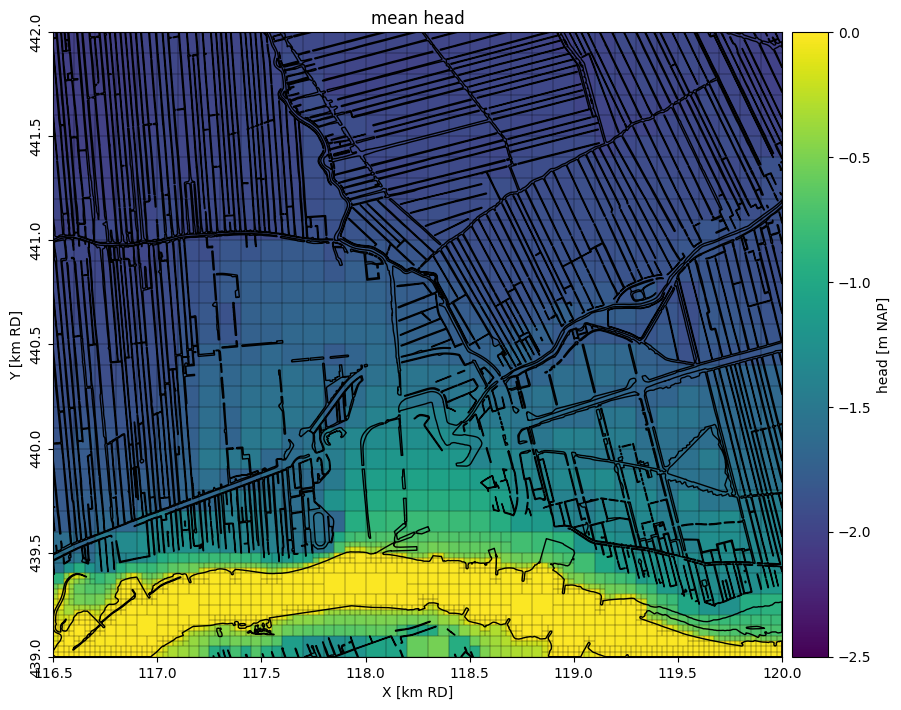
Plot the average head in the first layer on a map

norm = matplotlib.colors.Normalize(-2.5, 0.0)


pc = nlmod.plot.map_array(
    head.sel(layer="HLc").mean("time"),
    ds,
    norm=norm,
    colorbar=True,
    colorbar_label="head [m NAP]",
    title="mean head",
)
bgt.dissolve().plot(ax=pc.axes, edgecolor="k", facecolor="none");

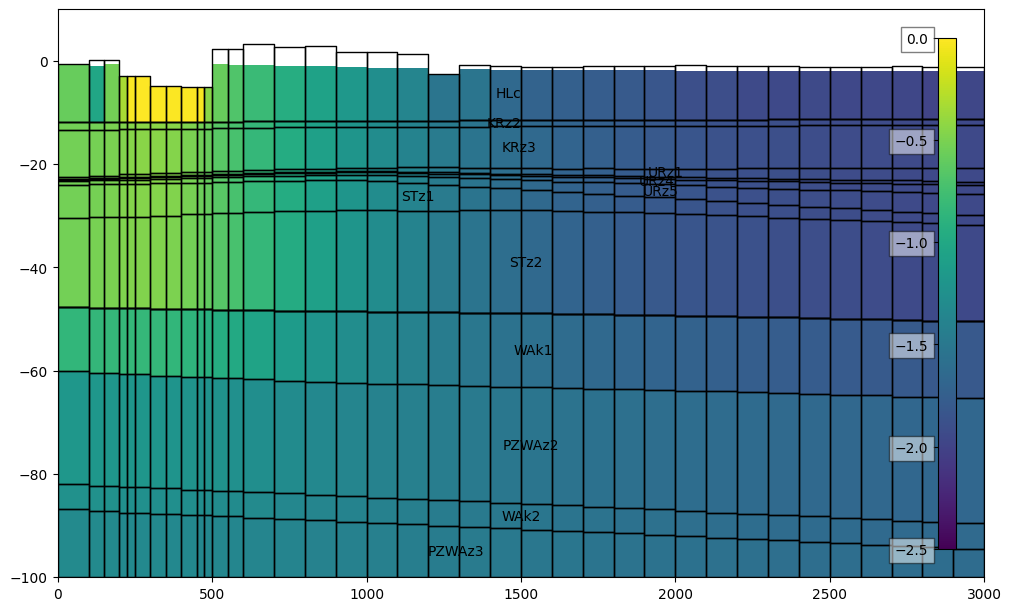
Plot the average head in a cross-section, from north to south

x = 118228.0
line = [(x, 439000), (x, 442000)]

f, ax = plt.subplots(figsize=(10, 6), layout="constrained")
dcs = DatasetCrossSection(ds, line, ax=ax, zmin=-100.0, zmax=10.0)
pc = dcs.plot_array(head.mean("time"), norm=norm, head=head.mean("time"))

# add labels with layer names
cbar = nlmod.plot.colorbar_inside(pc)
dcs.plot_grid()
dcs.plot_layers(colors="none", min_label_area=1000)

[<matplotlib.patches.Polygon at 0x7457b85aa550>,
 <matplotlib.patches.Polygon at 0x7457b85a9b50>,
 <matplotlib.patches.Polygon at 0x7457adf06990>,
 <matplotlib.patches.Polygon at 0x7457ae736350>,
 <matplotlib.patches.Polygon at 0x7457adfc5450>,
 <matplotlib.patches.Polygon at 0x7457aef69990>,
 <matplotlib.patches.Polygon at 0x7457ac79bf10>,
 <matplotlib.patches.Polygon at 0x7457ad35c650>,
 <matplotlib.patches.Polygon at 0x7457adb0dc90>,
 <matplotlib.patches.Polygon at 0x7457ad35db10>,
 <matplotlib.patches.Polygon at 0x7457aefa65d0>,
 <matplotlib.patches.Polygon at 0x7457aefa4c50>,
 <matplotlib.patches.Polygon at 0x7457aefa4410>,
 <matplotlib.patches.Polygon at 0x7457ae795c50>,
 <matplotlib.patches.Polygon at 0x7457ae716a90>,
 <matplotlib.patches.Polygon at 0x7457aefec9d0>]

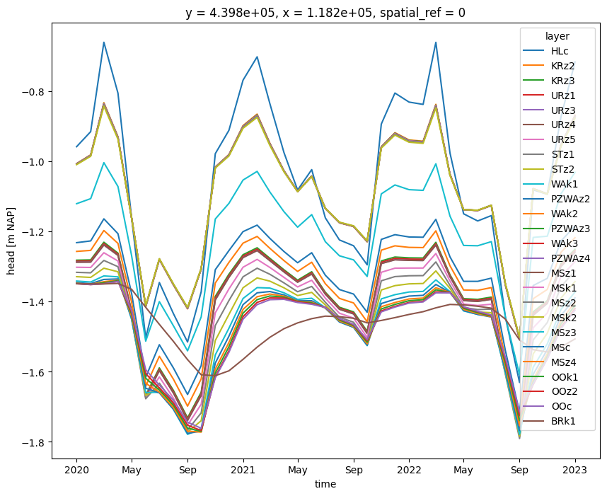
plot a time series at a certain location

x = 118228
y = 439870
head_point = nlmod.gwf.get_head_at_point(head, x=x, y=y, ds=ds)
fig, ax = plt.subplots(1, 1, figsize=(10, 8))
handles = head_point.plot.line(ax=ax, hue="layer")
ax.set_ylabel("head [m NAP]");

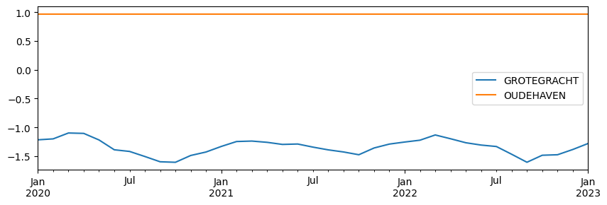
plot the lake stages

df = pd.read_csv(os.path.join(model_ws, "lak_STAGE.csv"), index_col=0)
df.index = ds.time.values
ax = df.plot(figsize=(10, 3))

Compare with BRO measurements

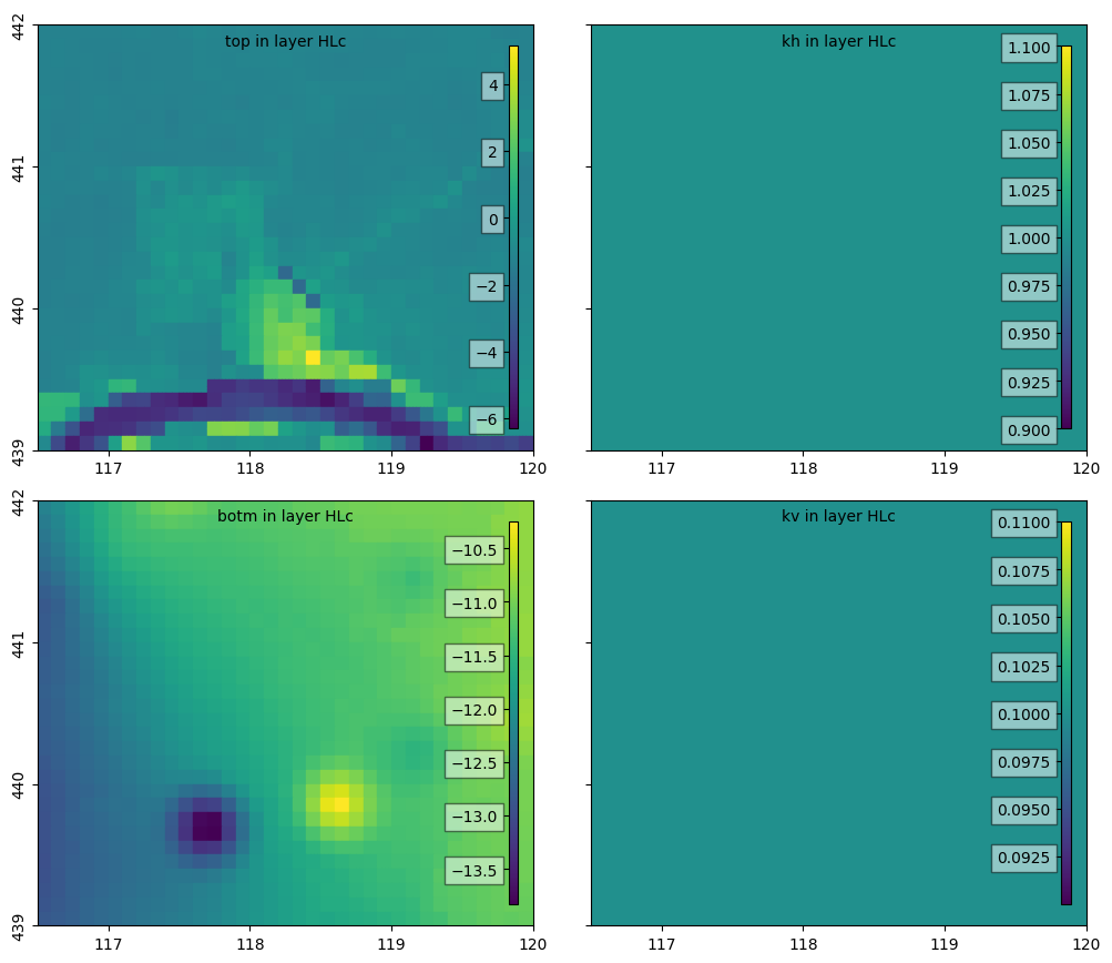
Plot some properties of the first layer

We can plot some properties of the first layer, called HLc. As REGIS does not contain data about hydraulic conductivities for this layer, default values of 1 m/d for kh and 0.1 m/d for hv are used, which can be seen in the graphs below.

layer = "HLc"

f, axes = nlmod.plot.get_map(extent, nrows=2, ncols=2)
variables = ["top", "kh", "botm", "kv"]
for i, variable in enumerate(variables):
    ax = axes.ravel()[i]
    if variable == "top":
        if layer == ds.layer[0]:
            da = ds["top"]
        else:
            da = ds["botm"][np.where(ds.layer == layer)[0][0] - 1]
    else:
        da = ds[variable].sel(layer=layer)
    pc = nlmod.plot.data_array(da, ds=ds, ax=ax)
    nlmod.plot.colorbar_inside(pc, ax=ax)
    ax.text(
        0.5,
        0.98,
        f"{variable} in layer {layer}",
        ha="center",
        va="top",
        transform=ax.transAxes,
    )

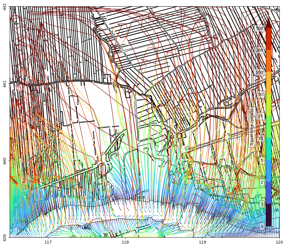
Add pathlines

We create a modpath model which calculates the pathlines. We calculate the pathlines that start in the center of the modflow cells with a river boundary condition (the cells in the “Lek” river).

# create a modpath model
mpf = nlmod.modpath.mpf(gwf)

# create the basic modpath package
_mpfbas = nlmod.modpath.bas(mpf)

# get the nodes from a package
nodes = nlmod.modpath.package_to_nodes(gwf, "RIV_0", ibound=mpf.ib)

# create a particle tracking group from cell centers
pg = nlmod.modpath.pg_from_pd(nodes, localx=0.5, localy=0.5, localz=0.5)

# create the modpath simulation file
mpsim = nlmod.modpath.sim(mpf, pg, "forward", gwf=gwf)

adding Package:  MPBAS
adding Package:  MPSIM

# run modpath model
nlmod.modpath.write_and_run(mpf)

INFO:nlmod.modpath.modpath.write_and_run:write modpath files to model workspace

Writing packages:
   Package:  MPBAS
   Package:  MPSIM
 
INFO:nlmod.modpath.modpath.write_and_run:run modpath model
FloPy is using the following executable to run the model: ../../../../../../envs/latest/lib/python3.11/site-packages/nlmod/bin/mp7_2_002_provisional

MODPATH Version 7.2.002 PROVISIONAL 
Program compiled Oct 16 2023 02:57:43 with IFORT compiler (ver. 20.21.7)
 
Run particle tracking simulation ...
Processing Time Step     1 Period     1.  Time =  3.65200E+03  Steady-state flow
Processing Time Step     1 Period     2.  Time =  3.68300E+03  Steady-state flow                                                    
Processing Time Step     1 Period     3.  Time =  3.71200E+03  Steady-state flow                                                    
Processing Time Step     1 Period     4.  Time =  3.74300E+03  Steady-state flow                                                    
Processing Time Step     1 Period     5.  Time =  3.77300E+03  Steady-state flow                                                    
Processing Time Step     1 Period     6.  Time =  3.80400E+03  Steady-state flow
Processing Time Step     1 Period     7.  Time =  3.83400E+03  Steady-state flow                                                    
Processing Time Step     1 Period     8.  Time =  3.86500E+03  Steady-state flow                                                    
Processing Time Step     1 Period     9.  Time =  3.89600E+03  Steady-state flow                                                    
Processing Time Step     1 Period    10.  Time =  3.92600E+03  Steady-state flow                                                    
Processing Time Step     1 Period    11.  Time =  3.95700E+03  Steady-state flow
Processing Time Step     1 Period    12.  Time =  3.98700E+03  Steady-state flow                                                    
Processing Time Step     1 Period    13.  Time =  4.01800E+03  Steady-state flow                                                    
Processing Time Step     1 Period    14.  Time =  4.04900E+03  Steady-state flow                                                    
Processing Time Step     1 Period    15.  Time =  4.07700E+03  Steady-state flow                                                    
Processing Time Step     1 Period    16.  Time =  4.10800E+03  Steady-state flow
Processing Time Step     1 Period    17.  Time =  4.13800E+03  Steady-state flow                                                    
Processing Time Step     1 Period    18.  Time =  4.16900E+03  Steady-state flow                                                    
Processing Time Step     1 Period    19.  Time =  4.19900E+03  Steady-state flow                                                    
Processing Time Step     1 Period    20.  Time =  4.23000E+03  Steady-state flow                                                    
Processing Time Step     1 Period    21.  Time =  4.26100E+03  Steady-state flow
Processing Time Step     1 Period    22.  Time =  4.29100E+03  Steady-state flow                                                    
Processing Time Step     1 Period    23.  Time =  4.32200E+03  Steady-state flow                                                    
Processing Time Step     1 Period    24.  Time =  4.35200E+03  Steady-state flow                                                    
Processing Time Step     1 Period    25.  Time =  4.38300E+03  Steady-state flow                                                    
Processing Time Step     1 Period    26.  Time =  4.41400E+03  Steady-state flow
Processing Time Step     1 Period    27.  Time =  4.44200E+03  Steady-state flow                                                    
Processing Time Step     1 Period    28.  Time =  4.47300E+03  Steady-state flow                                                    
Processing Time Step     1 Period    29.  Time =  4.50300E+03  Steady-state flow                                                    
Processing Time Step     1 Period    30.  Time =  4.53400E+03  Steady-state flow                                                    
Processing Time Step     1 Period    31.  Time =  4.56400E+03  Steady-state flow
Processing Time Step     1 Period    32.  Time =  4.59500E+03  Steady-state flow                                                    
Processing Time Step     1 Period    33.  Time =  4.62600E+03  Steady-state flow                                                    
Processing Time Step     1 Period    34.  Time =  4.65600E+03  Steady-state flow                                                    
Processing Time Step     1 Period    35.  Time =  4.68700E+03  Steady-state flow                                                    
Processing Time Step     1 Period    36.  Time =  4.71700E+03  Steady-state flow
Processing Time Step     1 Period    37.  Time =  4.74800E+03  Steady-state flow

Particle Summary:
         0 particles are pending release.
         0 particles remain active.
         0 particles terminated at boundary faces.
         0 particles terminated at weak sink cells.
         0 particles terminated at weak source cells.
       999 particles terminated at strong source/sink cells.
         0 particles terminated in cells with a specified zone number.
         0 particles were stranded in inactive or dry cells.
         0 particles were unreleased.
         0 particles have an unknown status.
 
Normal termination.

pdata = nlmod.modpath.load_pathline_data(mpf)

def get_segments(x, y, segments=None):
    # split each flow path into multiple line segments
    return [np.column_stack([x[i : i + 2], y[i : i + 2]]) for i in range(len(x) - 1)]


def get_array(time, to_year=True):
    # for each line-segment use the average time as the color
    array = (time[:-1] + time[1:]) / 2
    if to_year:
        array = array / 365.25
    return array


cmap = plt.get_cmap("turbo")
norm = matplotlib.colors.BoundaryNorm(
    [0, 1, 2, 5, 10, 25, 50, 100, 200, 500], cmap.N, extend="max"
)

# get line segments and color values
segments = []
array = []
for pid in np.unique(pdata["particleid"]):
    pf = pdata[pdata["particleid"] == pid]
    segments.extend(get_segments(pf["x"], pf["y"]))
    array.extend(get_array(pf["time"]))

f, ax = nlmod.plot.get_map(extent)
lc = matplotlib.collections.LineCollection(
    segments, cmap=cmap, norm=norm, array=array, linewidth=1.0
)
line = ax.add_collection(lc)
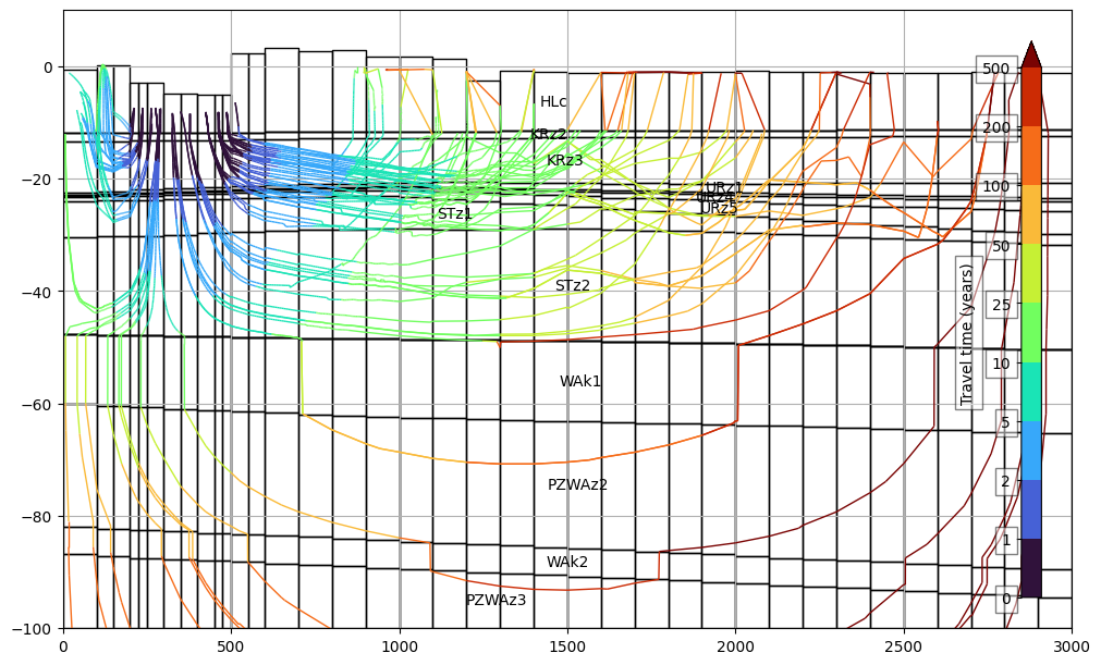
nlmod.plot.colorbar_inside(line, label="Travel time (years)")

bgt.dissolve().plot(ax=ax, edgecolor="k", facecolor="none");

x = 118228.0
line = LineString([(x, 439000), (x, 442000)])

# get line segments and color values
segments = []
array = []
for pid in np.unique(pdata["particleid"]):
    pf = pdata[pdata["particleid"] == pid]
    d = line.distance(Point(pf["x"][0], pf["y"][0]))
    if d < 200.0:
        x = [line.project(Point(x, y)) for x, y in zip(pf["x"], pf["y"])]
        segments.extend(get_segments(x, pf["z"]))
        array.extend(get_array(pf["time"]))

f, ax = plt.subplots(figsize=(10, 6), layout="constrained")
ax.grid()
dcs = DatasetCrossSection(ds, line, ax=ax, zmin=-100.0, zmax=10.0)
lc = matplotlib.collections.LineCollection(
    segments, cmap=cmap, norm=norm, array=array, linewidth=1.0
)
line = ax.add_collection(lc)
nlmod.plot.colorbar_inside(line, label="Travel time (years)")
# add grid
dcs.plot_grid()
# add labels with layer names
dcs.plot_layers(alpha=0.0, min_label_area=1000)

[<matplotlib.patches.Polygon at 0x745796835e90>,
 <matplotlib.patches.Polygon at 0x745796834e90>,
 <matplotlib.patches.Polygon at 0x7457ad7cdf10>,
 <matplotlib.patches.Polygon at 0x7457ad7cd450>,
 <matplotlib.patches.Polygon at 0x745796811350>,
 <matplotlib.patches.Polygon at 0x7457a93ab350>,
 <matplotlib.patches.Polygon at 0x7457a49b2390>,
 <matplotlib.patches.Polygon at 0x7457a49b2110>,
 <matplotlib.patches.Polygon at 0x7457a49ab1d0>,
 <matplotlib.patches.Polygon at 0x7457a49b0990>,
 <matplotlib.patches.Polygon at 0x7457a4989850>,
 <matplotlib.patches.Polygon at 0x7457a49a1250>,
 <matplotlib.patches.Polygon at 0x7457a49a3e50>,
 <matplotlib.patches.Polygon at 0x7457a4a6d410>,
 <matplotlib.patches.Polygon at 0x7457a4a6d010>,
 <matplotlib.patches.Polygon at 0x7457a4a6fa50>]