Aggregating surface water

In nlmod, surface water is mostly added to a groundwater model using a GeoDataFrame with surface water features. nlmod can generate input from this GeoDataFrame for the DRN- RIV or LAK-packages. Each individual record can directly be added to these packages. Aggregation of surface water features in cells is also possible, using different aggregation-methods.

This section demonstrates how to aggrgate surface water features into model cells and add them to a MODFLOW model. In this notebook we perform a steady-state run, in which the stage of the surface water is the mean of the summer and winter stage. The surface water bodies in each cell are aggregated using an area-weighted method and added to the model with the river-package.

import os
import matplotlib.pyplot as plt
import pandas as pd
import geopandas as gpd
import flopy
import nlmod

Model settings

We define some model settings, like the name, the directory of the model files, the model extent and the time

model_name = "Schoonhoven"
model_ws = "03_aggregating_surface_water"
figdir, cachedir = nlmod.util.get_model_dirs(model_ws)
extent = [116_500, 120_000, 439_000, 442_000]
time = pd.date_range("2020", "2023", freq="MS")  # monthly timestep

layer ‘waterdeel’ from bgt

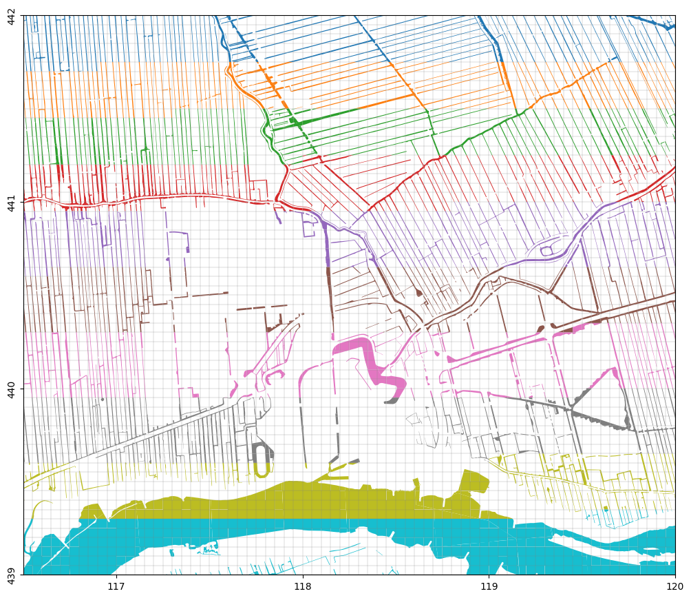
The location of the surface water bodies is obtained from the GeoDataFrame that was created in the the surface water notebook. We saved this data as a geosjon file and load it here.

fname_bgt = os.path.join("..", "data_sources", "02_surface_water", "cache", "bgt.gpkg")
if not os.path.isfile(fname_bgt):
    raise (
        Exception(
            f"{fname_bgt} not found. Please run notebook 02_surface_water.ipynb in the 'data_sources' directory first"
        )
    )
bgt = gpd.read_file(fname_bgt)

Change some values in the GeoDataFrame for this model

sfw = bgt
sfw["stage"] = sfw[["winter_stage", "summer_stage"]].mean(1)
# use a water depth of 0.5 meter
sfw["botm"] = sfw["stage"] - 0.5
# set the stage of the Lek to 0.0 m NAP and the botm to -3 m NAP
mask = sfw["bronhouder"] == "L0002"
sfw.loc[mask, "stage"] = 0.0
sfw.loc[mask, "botm"] = -3.0

Take a look at the first few rows. For adding surface water features to a MODFLOW model the following attributes must be present:

• stage: the water level (in m NAP)

• botm: the bottom elevation (in m NAP)

• c0: the bottom resistance (in days)

The stage and the botm columns are present in our dataset. The bottom resistance c0 is rarely known, and is usually estimated when building the model. We will add our estimate later on.

Note

The NaN’s in the dataset indicate that not all parameters are known for each feature. This is not necessarily a problem but this will mean some features will not be converted to model input.

Now use stage as the column to color the data. Note the missing features caused by the fact that the stage is undefined (NaN).

fig, ax = nlmod.plot.get_map(extent)
sfw.plot(ax=ax, column="stage", legend=True);

Build model

The next step is to define a model grid and build a model (i.e. create a discretization and define flow parameters).

Build the model. We’re keeping the model as simple as possible.

delr = delc = 50.0
start_time = "2021-01-01"

# layer model
layer_model = nlmod.read.download_regis(
    extent, cachedir=cachedir, cachename="layer_model.nc"
)
layer_model

Botm of layer is not equal to top of deeper layer in 3 cells

<xarray.Dataset> Size: 371kB
Dimensions:      (y: 30, x: 35, layer: 29)
Coordinates:
  * y            (y) float64 240B 4.42e+05 4.418e+05 ... 4.392e+05 4.39e+05
  * x            (x) float64 280B 1.166e+05 1.166e+05 ... 1.198e+05 1.2e+05
  * layer        (layer) <U8 928B 'HLc' 'KRWYk1' 'KRz2' ... 'OOz2' 'OOc' 'BRk1'
    spatial_ref  int64 8B 0
Data variables:
    top          (y, x) float32 4kB -1.28 -1.22 -1.25 ... -4.05 -3.76 -4.21
    botm         (layer, y, x) float32 122kB -12.26 -12.11 ... -593.9 -595.5
    kh           (layer, y, x) float32 122kB nan nan nan nan ... nan nan nan nan
    kv           (layer, y, x) float32 122kB nan nan nan ... 0.002 0.002 0.002
Attributes: (12/41)
    references:                    https://www.dinoloket.nl/regis-ii-het-hydr...
    Conventions:                   CF-1.7
    creator_url:                   https://www.dinoloket.nl
    keywords_vocabulary:           NASA/GCMD Earth Science Keywords. Version 6.0
    acknowledgment:                https://www.dinoloket.nl
    project:                       REGIS v02r2s3
    ...                            ...
    geospatial_vertical_min:       -1235.92
    geospatial_vertical_max:       322.75
    geospatial_vertical_units:     m-NAP
    geospatial_vertical_positive:  up
    gridtype:                      structured
    extent:                        [116500, 120000, 439000, 442000]

xarray.Dataset

• Dimensions:
  • y: 30
  • x: 35
  • layer: 29
• Coordinates: (4)
  • y
    (y)
    float64
    4.42e+05 4.418e+05 ... 4.39e+05

    comment :

    y-coordinate values at the upper and lower bounds of each pixel.

    array([441950., 441850., 441750., 441650., 441550., 441450., 441350., 441250.,
           441150., 441050., 440950., 440850., 440750., 440650., 440550., 440450.,
           440350., 440250., 440150., 440050., 439950., 439850., 439750., 439650.,
           439550., 439450., 439350., 439250., 439150., 439050.])

  • x
    (x)
    float64
    1.166e+05 1.166e+05 ... 1.2e+05

    comment :

    x-coordinate values at the left and right bounds of each pixel.

    array([116550., 116650., 116750., 116850., 116950., 117050., 117150., 117250.,
           117350., 117450., 117550., 117650., 117750., 117850., 117950., 118050.,
           118150., 118250., 118350., 118450., 118550., 118650., 118750., 118850.,
           118950., 119050., 119150., 119250., 119350., 119450., 119550., 119650.,
           119750., 119850., 119950.])

  • layer
    (layer)
    <U8
    'HLc' 'KRWYk1' ... 'OOc' 'BRk1'

    array(['HLc', 'KRWYk1', 'KRz2', 'KRz3', 'URz1', 'URz3', 'URz4', 'URz5', 'STz1',
           'STz2', 'SYk1', 'PZWAz1', 'WAk1', 'PZWAz2', 'WAk2', 'PZWAz3', 'WAk3',
           'PZWAz4', 'MSz1', 'MSk1', 'MSz2', 'MSk2', 'MSz3', 'MSc', 'MSz4', 'OOk1',
           'OOz2', 'OOc', 'BRk1'], dtype='<U8')

  • spatial_ref
    ()
    int64
    0

    crs_wkt :

    PROJCS["Amersfoort / RD New",GEOGCS["Amersfoort",DATUM["Amersfoort",SPHEROID["Bessel 1841",6377397.155,299.1528128,AUTHORITY["EPSG","7004"]],AUTHORITY["EPSG","6289"]],PRIMEM["Greenwich",0,AUTHORITY["EPSG","8901"]],UNIT["degree",0.0174532925199433,AUTHORITY["EPSG","9122"]],AUTHORITY["EPSG","4289"]],PROJECTION["Oblique_Stereographic"],PARAMETER["latitude_of_origin",52.1561605555556],PARAMETER["central_meridian",5.38763888888889],PARAMETER["scale_factor",0.9999079],PARAMETER["false_easting",155000],PARAMETER["false_northing",463000],UNIT["metre",1,AUTHORITY["EPSG","9001"]],AXIS["Easting",EAST],AXIS["Northing",NORTH],AUTHORITY["EPSG","28992"]]

    spatial_ref :

    PROJCS["Amersfoort / RD New",GEOGCS["Amersfoort",DATUM["Amersfoort",SPHEROID["Bessel 1841",6377397.155,299.1528128,AUTHORITY["EPSG","7004"]],AUTHORITY["EPSG","6289"]],PRIMEM["Greenwich",0,AUTHORITY["EPSG","8901"]],UNIT["degree",0.0174532925199433,AUTHORITY["EPSG","9122"]],AUTHORITY["EPSG","4289"]],PROJECTION["Oblique_Stereographic"],PARAMETER["latitude_of_origin",52.1561605555556],PARAMETER["central_meridian",5.38763888888889],PARAMETER["scale_factor",0.9999079],PARAMETER["false_easting",155000],PARAMETER["false_northing",463000],UNIT["metre",1,AUTHORITY["EPSG","9001"]],AXIS["Easting",EAST],AXIS["Northing",NORTH],AUTHORITY["EPSG","28992"]]

    array(0)

• Data variables: (4)
  • top
    (y, x)
    float32
    -1.28 -1.22 -1.25 ... -3.76 -4.21

    long_name :

    top

    standard_name :

    depth_of_top_of_layer

    units :

    mNAP

    source :

    REGIS

    url :

    https://www.dinodata.nl/opendap/REGIS/REGIS.nc

    date :

    20260513

    array([[-1.28, -1.22, -1.25, ..., -1.24, -1.33, -1.26],
           [-1.26, -1.17, -1.24, ..., -1.11, -1.16, -1.3 ],
           [-1.29, -1.17, -1.27, ..., -1.  , -1.22, -1.3 ],
           ...,
           [ 1.17,  1.17, -0.1 , ..., -0.05,  0.15, -0.57],
           [ 0.69, -1.59, -3.38, ...,  1.18, -0.63, -0.66],
           [-0.91, -3.74, -5.36, ..., -4.05, -3.76, -4.21]],
          shape=(30, 35), dtype=float32)

  • botm
    (layer, y, x)
    float32
    -12.26 -12.11 ... -593.9 -595.5

    long_name :

    bottom

    standard_name :

    depth_of_bottom_of_layer

    units :

    mNAP

    source :

    REGIS

    url :

    https://www.dinodata.nl/opendap/REGIS/REGIS.nc

    date :

    20260513

    array([[[ -12.26,  -12.11,  -11.93, ...,  -10.96,  -10.87,  -10.84],
            [ -12.34,  -12.18,  -11.98, ...,  -10.89,  -10.87,  -10.84],
            [ -12.41,  -12.25,  -12.05, ...,  -10.9 ,  -10.87,  -10.84],
            ...,
            [ -12.92,  -12.86,  -12.74, ...,  -11.09,  -11.06,  -11.07],
            [ -12.89,  -12.83,  -12.76, ...,  -11.1 ,  -11.07,  -11.08],
            [ -12.85,  -12.8 ,  -12.74, ...,  -11.11,  -11.12,  -11.09]],
    
           [[ -12.26,  -12.11,  -11.93, ...,  -11.17,  -11.18,  -11.19],
            [ -12.34,  -12.18,  -11.98, ...,  -11.14,  -11.15,  -11.16],
            [ -12.41,  -12.25,  -12.05, ...,  -11.1 ,  -11.11,  -11.12],
            ...,
            [ -12.92,  -12.86,  -12.74, ...,  -11.09,  -11.06,  -11.07],
            [ -12.89,  -12.83,  -12.76, ...,  -11.1 ,  -11.07,  -11.08],
            [ -12.85,  -12.8 ,  -12.74, ...,  -11.11,  -11.12,  -11.09]],
    
           [[ -13.17,  -13.03,  -12.87, ...,  -12.06,  -11.97,  -11.94],
            [ -13.28,  -13.12,  -12.94, ...,  -12.03,  -12.  ,  -11.97],
            [ -13.37,  -13.21,  -13.02, ...,  -12.07,  -12.03,  -12.  ],
            ...,
    ...
            [-326.14, -326.17, -326.2 , ..., -325.79, -325.75, -325.71],
            [-326.19, -326.1 , -326.13, ..., -325.75, -325.71, -325.67],
            [-326.12, -326.15, -326.17, ..., -325.71, -325.67, -325.62]],
    
           [[-368.87, -368.48, -368.  , ..., -363.1 , -363.09, -363.06],
            [-368.44, -367.94, -367.44, ..., -362.64, -362.64, -362.64],
            [-368.1 , -367.41, -366.89, ..., -362.21, -362.23, -362.23],
            ...,
            [-365.17, -364.72, -364.16, ..., -359.84, -359.92, -359.97],
            [-365.63, -365.07, -364.58, ..., -360.09, -360.12, -360.15],
            [-365.99, -365.36, -364.97, ..., -360.37, -360.39, -360.4 ]],
    
           [[-502.26, -503.93, -505.66, ..., -551.66, -553.08, -554.67],
            [-502.73, -504.44, -506.24, ..., -553.3 , -554.7 , -556.21],
            [-503.26, -505.03, -506.88, ..., -554.88, -556.22, -557.84],
            ...,
            [-532.1 , -533.2 , -534.37, ..., -593.62, -594.94, -595.81],
            [-532.73, -533.75, -534.87, ..., -593.  , -594.45, -595.98],
            [-533.32, -534.27, -535.31, ..., -592.32, -593.89, -595.55]]],
          shape=(29, 30, 35), dtype=float32)

  • kh
    (layer, y, x)
    float32
    nan nan nan nan ... nan nan nan nan

    long_name :

    kh

    standard_name :

    horizontale_doorlatendheid_(kh)

    units :

    m/day

    source :

    REGIS

    url :

    https://www.dinodata.nl/opendap/REGIS/REGIS.nc

    date :

    20260513

    array([[[  nan,   nan,   nan, ...,   nan,   nan,   nan],
            [  nan,   nan,   nan, ...,   nan,   nan,   nan],
            [  nan,   nan,   nan, ...,   nan,   nan,   nan],
            ...,
            [  nan,   nan,   nan, ...,   nan,   nan,   nan],
            [  nan,   nan,   nan, ...,   nan,   nan,   nan],
            [  nan,   nan,   nan, ...,   nan,   nan,   nan]],
    
           [[  nan,   nan,   nan, ...,   nan,   nan,   nan],
            [  nan,   nan,   nan, ...,   nan,   nan,   nan],
            [  nan,   nan,   nan, ...,   nan,   nan,   nan],
            ...,
            [  nan,   nan,   nan, ...,   nan,   nan,   nan],
            [  nan,   nan,   nan, ...,   nan,   nan,   nan],
            [  nan,   nan,   nan, ...,   nan,   nan,   nan]],
    
           [[56.61, 57.18, 57.66, ..., 38.27, 37.81, 37.36],
            [55.45, 56.04, 56.51, ..., 37.59, 37.05, 36.65],
            [54.2 , 54.8 , 55.33, ..., 36.9 , 36.88, 36.04],
            ...,
    ...
            [ 7.86,  7.84,  7.82, ...,  7.47,  7.48,  7.48],
            [ 7.86,  7.84,  7.73, ...,  7.46,  7.45,  7.45],
            [ 7.88,  7.83,  7.72, ...,  7.43,  7.42,  7.42]],
    
           [[ 1.21,  1.21,  1.21, ...,  1.25,  1.25,  1.26],
            [ 1.21,  1.21,  1.21, ...,  1.26,  1.26,  1.27],
            [ 1.22,  1.21,  1.21, ...,  1.27,  1.26,  1.28],
            ...,
            [ 1.34,  1.34,  1.34, ...,  1.43,  1.43,  1.44],
            [ 1.35,  1.36,  1.35, ...,  1.42,  1.43,  1.43],
            [ 1.37,  1.37,  1.37, ...,  1.41,  1.42,  1.43]],
    
           [[  nan,   nan,   nan, ...,   nan,   nan,   nan],
            [  nan,   nan,   nan, ...,   nan,   nan,   nan],
            [  nan,   nan,   nan, ...,   nan,   nan,   nan],
            ...,
            [  nan,   nan,   nan, ...,   nan,   nan,   nan],
            [  nan,   nan,   nan, ...,   nan,   nan,   nan],
            [  nan,   nan,   nan, ...,   nan,   nan,   nan]]],
          shape=(29, 30, 35), dtype=float32)

  • kv
    (layer, y, x)
    float32
    nan nan nan ... 0.002 0.002 0.002

    long_name :

    kv

    standard_name :

    verticale_doorlatendheid_(kv)

    units :

    m/day

    source :

    REGIS

    url :

    https://www.dinodata.nl/opendap/REGIS/REGIS.nc

    date :

    20260513

    array([[[       nan,        nan,        nan, ...,        nan,
                    nan,        nan],
            [       nan,        nan,        nan, ...,        nan,
                    nan,        nan],
            [       nan,        nan,        nan, ...,        nan,
                    nan,        nan],
            ...,
            [       nan,        nan,        nan, ...,        nan,
                    nan,        nan],
            [       nan,        nan,        nan, ...,        nan,
                    nan,        nan],
            [       nan,        nan,        nan, ...,        nan,
                    nan,        nan]],
    
           [[       nan,        nan,        nan, ..., 0.01483528,
             0.01504688, 0.01521849],
            [       nan,        nan,        nan, ..., 0.01478147,
             0.01492398, 0.01504013],
            [       nan,        nan,        nan, ..., 0.01469031,
             0.01487229, 0.01486955],
    ...
            [0.0071571 , 0.00716144, 0.00716829, ..., 0.00776395,
             0.00780907, 0.00788237],
            [0.00720632, 0.00721143, 0.0072237 , ..., 0.00784941,
             0.00793054, 0.00801546],
            [0.00724916, 0.00725398, 0.00726712, ..., 0.00794574,
             0.00802989, 0.00812249]],
    
           [[0.002     , 0.002     , 0.002     , ..., 0.002     ,
             0.002     , 0.002     ],
            [0.002     , 0.002     , 0.002     , ..., 0.002     ,
             0.002     , 0.002     ],
            [0.002     , 0.002     , 0.002     , ..., 0.002     ,
             0.002     , 0.002     ],
            ...,
            [0.002     , 0.002     , 0.002     , ..., 0.002     ,
             0.002     , 0.002     ],
            [0.002     , 0.002     , 0.002     , ..., 0.002     ,
             0.002     , 0.002     ],
            [0.002     , 0.002     , 0.002     , ..., 0.002     ,
             0.002     , 0.002     ]]], shape=(29, 30, 35), dtype=float32)

• Attributes: (41)

  references :

  https://www.dinoloket.nl/regis-ii-het-hydrogeologische-model

  Conventions :

  CF-1.7

  creator_url :

  https://www.dinoloket.nl

  keywords_vocabulary :

  NASA/GCMD Earth Science Keywords. Version 6.0

  acknowledgment :

  https://www.dinoloket.nl

  project :

  REGIS v02r2s3

  creator_name :

  Geological Survey of the Netherlands, part of TNO

  cdm_data_type :

  grid

  featureType :

  grid

  summary :

  The Digital Geological Model DGM is used as the basis for the regional hydrogeological model REGIS II, serving as the starting point for further subdivision of the modelled geological units into hydrogeological units, aquifers and aquitards. Using the lithological information from boreholes and additional hydrological data such as hydraulic heads and pumping tests, the hydrogeological units are characterised in terms of their hydraulic conductivity, transmissivity and vertical resistivity, vertical flow resistance. To ensure consistency between the geological and hydrogeological models, the hydrogeological units are constrained within the units of DGM. The depths to the top and the base, and the thickness of the units have been mapped in grid files at 100 x 100 metres resolution.

  license :

  cc-by-

  publisher_name :

  TNO

  creator_email :

  info@dinoloket.nl

  keywords :

  lithological classes, tops and bottoms of layers, transmissivity

  institution :

  TNO

  history :

  www.dinoloket.nl

  naming_authority :

  dinoloket.nl

  source :

  www.dinoloket.nl

  publisher_url :

  www.dinoloket.nl

  publisher_email :

  info@dinoloket.nl

  Metadata_Conventions :

  Unidata Dataset Discovery v1.0

  standard_name_vocabulary :

  CF-1.6

  title :

  REGIS v02r2s3

  id :

  7fd8576c-b6c0-4b13-a743-7a0c47df4b29

  date_created :

  2024-12-19T20:44:07Z

  date_modified :

  2024-12-19T20:44:07Z

  date_issued :

  2024-12-19T20:44:07Z

  geospatial_lat_min :

  50.669197

  geospatial_lat_max :

  53.638645

  geospatial_lat_units :

  degrees_north

  geospatial_lat_resolution :

  0.0008998327

  geospatial_lon_min :

  3.1946514

  geospatial_lon_max :

  7.428299

  geospatial_lon_units :

  degrees_east

  geospatial_lon_resolution :

  0.0014598784

  geospatial_vertical_min :

  -1235.92

  geospatial_vertical_max :

  322.75

  geospatial_vertical_units :

  m-NAP

  geospatial_vertical_positive :

  up

  gridtype :

  structured

  extent :

  [116500, 120000, 439000, 442000]

# create a model ds by changing grid of layer_model
ds = nlmod.to_model_ds(layer_model, model_name, model_ws, delr=delr, delc=delc)

# create model time dataset
ds = nlmod.time.set_ds_time(ds, start=start_time, steady=True, perlen=1)

ds

<xarray.Dataset> Size: 2MB
Dimensions:      (y: 60, x: 70, layer: 29, time: 1)
Coordinates:
  * y            (y) float64 480B 4.42e+05 4.419e+05 ... 4.391e+05 4.39e+05
  * x            (x) float64 560B 1.165e+05 1.166e+05 ... 1.199e+05 1.2e+05
  * layer        (layer) <U8 928B 'HLc' 'KRWYk1' 'KRz2' ... 'OOz2' 'OOc' 'BRk1'
  * time         (time) datetime64[ns] 8B 2021-01-02
    spatial_ref  int64 8B 0
Data variables:
    top          (y, x) float32 17kB -1.28 -1.28 -1.22 ... -3.76 -4.21 -4.21
    botm         (layer, y, x) float32 487kB -12.26 -12.26 ... -595.5 -595.5
    kh           (layer, y, x) float32 487kB 1.0 1.0 1.0 1.0 ... 0.02 0.02 0.02
    kv           (layer, y, x) float32 487kB 0.1 0.1 0.1 ... 0.002 0.002 0.002
    area         (y, x) float64 34kB 2.5e+03 2.5e+03 2.5e+03 ... 2.5e+03 2.5e+03
    steady       (time) int64 8B 1
    nstp         (time) int64 8B 1
    tsmult       (time) float64 8B 1.0
Attributes:
    extent:      [116500, 120000, 439000, 442000]
    gridtype:    structured
    model_name:  Schoonhoven
    mfversion:   mf6
    created_on:  20260513_15:16:24
    exe_name:    /home/docs/checkouts/readthedocs.org/user_builds/nlmod/envs/...
    model_ws:    03_aggregating_surface_water
    figdir:      03_aggregating_surface_water/figure
    cachedir:    03_aggregating_surface_water/cache
    transport:   0

xarray.Dataset

• Dimensions:
  • y: 60
  • x: 70
  • layer: 29
  • time: 1
• Coordinates: (5)
  • y
    (y)
    float64
    4.42e+05 4.419e+05 ... 4.39e+05

    comment :

    y-coordinate values at the upper and lower bounds of each pixel.

    array([441975., 441925., 441875., 441825., 441775., 441725., 441675., 441625.,
           441575., 441525., 441475., 441425., 441375., 441325., 441275., 441225.,
           441175., 441125., 441075., 441025., 440975., 440925., 440875., 440825.,
           440775., 440725., 440675., 440625., 440575., 440525., 440475., 440425.,
           440375., 440325., 440275., 440225., 440175., 440125., 440075., 440025.,
           439975., 439925., 439875., 439825., 439775., 439725., 439675., 439625.,
           439575., 439525., 439475., 439425., 439375., 439325., 439275., 439225.,
           439175., 439125., 439075., 439025.])

  • x
    (x)
    float64
    1.165e+05 1.166e+05 ... 1.2e+05

    comment :

    x-coordinate values at the left and right bounds of each pixel.

    array([116525., 116575., 116625., 116675., 116725., 116775., 116825., 116875.,
           116925., 116975., 117025., 117075., 117125., 117175., 117225., 117275.,
           117325., 117375., 117425., 117475., 117525., 117575., 117625., 117675.,
           117725., 117775., 117825., 117875., 117925., 117975., 118025., 118075.,
           118125., 118175., 118225., 118275., 118325., 118375., 118425., 118475.,
           118525., 118575., 118625., 118675., 118725., 118775., 118825., 118875.,
           118925., 118975., 119025., 119075., 119125., 119175., 119225., 119275.,
           119325., 119375., 119425., 119475., 119525., 119575., 119625., 119675.,
           119725., 119775., 119825., 119875., 119925., 119975.])

  • layer
    (layer)
    <U8
    'HLc' 'KRWYk1' ... 'OOc' 'BRk1'

    array(['HLc', 'KRWYk1', 'KRz2', 'KRz3', 'URz1', 'URz3', 'URz4', 'URz5', 'STz1',
           'STz2', 'SYk1', 'PZWAz1', 'WAk1', 'PZWAz2', 'WAk2', 'PZWAz3', 'WAk3',
           'PZWAz4', 'MSz1', 'MSk1', 'MSz2', 'MSk2', 'MSz3', 'MSc', 'MSz4', 'OOk1',
           'OOz2', 'OOc', 'BRk1'], dtype='<U8')

  • time
    (time)
    datetime64[ns]
    2021-01-02

    name :

    Time

    description :

    End time of the stress period

    time_units :

    DAYS

    start :

    2021-01-01 00:00:00

    array(['2021-01-02T00:00:00.000000000'], dtype='datetime64[ns]')

  • spatial_ref
    ()
    int64
    0

    crs_wkt :

    PROJCS["Amersfoort / RD New",GEOGCS["Amersfoort",DATUM["Amersfoort",SPHEROID["Bessel 1841",6377397.155,299.1528128,AUTHORITY["EPSG","7004"]],AUTHORITY["EPSG","6289"]],PRIMEM["Greenwich",0,AUTHORITY["EPSG","8901"]],UNIT["degree",0.0174532925199433,AUTHORITY["EPSG","9122"]],AUTHORITY["EPSG","4289"]],PROJECTION["Oblique_Stereographic"],PARAMETER["latitude_of_origin",52.1561605555556],PARAMETER["central_meridian",5.38763888888889],PARAMETER["scale_factor",0.9999079],PARAMETER["false_easting",155000],PARAMETER["false_northing",463000],UNIT["metre",1,AUTHORITY["EPSG","9001"]],AXIS["Easting",EAST],AXIS["Northing",NORTH],AUTHORITY["EPSG","28992"]]

    spatial_ref :

    PROJCS["Amersfoort / RD New",GEOGCS["Amersfoort",DATUM["Amersfoort",SPHEROID["Bessel 1841",6377397.155,299.1528128,AUTHORITY["EPSG","7004"]],AUTHORITY["EPSG","6289"]],PRIMEM["Greenwich",0,AUTHORITY["EPSG","8901"]],UNIT["degree",0.0174532925199433,AUTHORITY["EPSG","9122"]],AUTHORITY["EPSG","4289"]],PROJECTION["Oblique_Stereographic"],PARAMETER["latitude_of_origin",52.1561605555556],PARAMETER["central_meridian",5.38763888888889],PARAMETER["scale_factor",0.9999079],PARAMETER["false_easting",155000],PARAMETER["false_northing",463000],UNIT["metre",1,AUTHORITY["EPSG","9001"]],AXIS["Easting",EAST],AXIS["Northing",NORTH],AUTHORITY["EPSG","28992"]]

    array(0)

• Data variables: (8)
  • top
    (y, x)
    float32
    -1.28 -1.28 -1.22 ... -4.21 -4.21

    long_name :

    top

    standard_name :

    depth_of_top_of_layer

    units :

    mNAP

    source :

    REGIS

    url :

    https://www.dinodata.nl/opendap/REGIS/REGIS.nc

    date :

    20260513

    array([[-1.28, -1.28, -1.22, ..., -1.33, -1.26, -1.26],
           [-1.28, -1.28, -1.22, ..., -1.33, -1.26, -1.26],
           [-1.26, -1.26, -1.17, ..., -1.16, -1.3 , -1.3 ],
           ...,
           [ 0.69,  0.69, -1.59, ..., -0.63, -0.66, -0.66],
           [-0.91, -0.91, -3.74, ..., -3.76, -4.21, -4.21],
           [-0.91, -0.91, -3.74, ..., -3.76, -4.21, -4.21]],
          shape=(60, 70), dtype=float32)

  • botm
    (layer, y, x)
    float32
    -12.26 -12.26 ... -595.5 -595.5

    long_name :

    bottom

    standard_name :

    depth_of_bottom_of_layer

    units :

    mNAP

    source :

    REGIS

    url :

    https://www.dinodata.nl/opendap/REGIS/REGIS.nc

    date :

    20260513

    array([[[ -12.26,  -12.26,  -12.11, ...,  -10.87,  -10.84,  -10.84],
            [ -12.26,  -12.26,  -12.11, ...,  -10.87,  -10.84,  -10.84],
            [ -12.34,  -12.34,  -12.18, ...,  -10.87,  -10.84,  -10.84],
            ...,
            [ -12.89,  -12.89,  -12.83, ...,  -11.07,  -11.08,  -11.08],
            [ -12.85,  -12.85,  -12.8 , ...,  -11.12,  -11.09,  -11.09],
            [ -12.85,  -12.85,  -12.8 , ...,  -11.12,  -11.09,  -11.09]],
    
           [[ -12.26,  -12.26,  -12.11, ...,  -11.18,  -11.19,  -11.19],
            [ -12.26,  -12.26,  -12.11, ...,  -11.18,  -11.19,  -11.19],
            [ -12.34,  -12.34,  -12.18, ...,  -11.15,  -11.16,  -11.16],
            ...,
            [ -12.89,  -12.89,  -12.83, ...,  -11.07,  -11.08,  -11.08],
            [ -12.85,  -12.85,  -12.8 , ...,  -11.12,  -11.09,  -11.09],
            [ -12.85,  -12.85,  -12.8 , ...,  -11.12,  -11.09,  -11.09]],
    
           [[ -13.17,  -13.17,  -13.03, ...,  -11.97,  -11.94,  -11.94],
            [ -13.17,  -13.17,  -13.03, ...,  -11.97,  -11.94,  -11.94],
            [ -13.28,  -13.28,  -13.12, ...,  -12.  ,  -11.97,  -11.97],
            ...,
    ...
            [-326.19, -326.19, -326.1 , ..., -325.71, -325.67, -325.67],
            [-326.12, -326.12, -326.15, ..., -325.67, -325.62, -325.62],
            [-326.12, -326.12, -326.15, ..., -325.67, -325.62, -325.62]],
    
           [[-368.87, -368.87, -368.48, ..., -363.09, -363.06, -363.06],
            [-368.87, -368.87, -368.48, ..., -363.09, -363.06, -363.06],
            [-368.44, -368.44, -367.94, ..., -362.64, -362.64, -362.64],
            ...,
            [-365.63, -365.63, -365.07, ..., -360.12, -360.15, -360.15],
            [-365.99, -365.99, -365.36, ..., -360.39, -360.4 , -360.4 ],
            [-365.99, -365.99, -365.36, ..., -360.39, -360.4 , -360.4 ]],
    
           [[-502.26, -502.26, -503.93, ..., -553.08, -554.67, -554.67],
            [-502.26, -502.26, -503.93, ..., -553.08, -554.67, -554.67],
            [-502.73, -502.73, -504.44, ..., -554.7 , -556.21, -556.21],
            ...,
            [-532.73, -532.73, -533.75, ..., -594.45, -595.98, -595.98],
            [-533.32, -533.32, -534.27, ..., -593.89, -595.55, -595.55],
            [-533.32, -533.32, -534.27, ..., -593.89, -595.55, -595.55]]],
          shape=(29, 60, 70), dtype=float32)

  • kh
    (layer, y, x)
    float32
    1.0 1.0 1.0 1.0 ... 0.02 0.02 0.02

    long_name :

    kh

    standard_name :

    horizontale_doorlatendheid_(kh)

    units :

    m/day

    source :

    REGIS

    url :

    https://www.dinodata.nl/opendap/REGIS/REGIS.nc

    date :

    20260513

    array([[[1.0000000e+00, 1.0000000e+00, 1.0000000e+00, ...,
             1.0000000e+00, 1.0000000e+00, 1.0000000e+00],
            [1.0000000e+00, 1.0000000e+00, 1.0000000e+00, ...,
             1.0000000e+00, 1.0000000e+00, 1.0000000e+00],
            [1.0000000e+00, 1.0000000e+00, 1.0000000e+00, ...,
             1.0000000e+00, 1.0000000e+00, 1.0000000e+00],
            ...,
            [1.0000000e+00, 1.0000000e+00, 1.0000000e+00, ...,
             1.0000000e+00, 1.0000000e+00, 1.0000000e+00],
            [1.0000000e+00, 1.0000000e+00, 1.0000000e+00, ...,
             1.0000000e+00, 1.0000000e+00, 1.0000000e+00],
            [1.0000000e+00, 1.0000000e+00, 1.0000000e+00, ...,
             1.0000000e+00, 1.0000000e+00, 1.0000000e+00]],
    
           [[1.0000000e+00, 1.0000000e+00, 1.0000000e+00, ...,
             1.5046880e-01, 1.5218490e-01, 1.5218490e-01],
            [1.0000000e+00, 1.0000000e+00, 1.0000000e+00, ...,
             1.5046880e-01, 1.5218490e-01, 1.5218490e-01],
            [1.0000000e+00, 1.0000000e+00, 1.0000000e+00, ...,
             1.4923981e-01, 1.5040131e-01, 1.5040131e-01],
    ...
             1.4299999e+00, 1.4299999e+00, 1.4299999e+00],
            [1.3700000e+00, 1.3700000e+00, 1.3700000e+00, ...,
             1.4200000e+00, 1.4299999e+00, 1.4299999e+00],
            [1.3700000e+00, 1.3700000e+00, 1.3700000e+00, ...,
             1.4200000e+00, 1.4299999e+00, 1.4299999e+00]],
    
           [[2.0000001e-02, 2.0000001e-02, 2.0000001e-02, ...,
             2.0000001e-02, 2.0000001e-02, 2.0000001e-02],
            [2.0000001e-02, 2.0000001e-02, 2.0000001e-02, ...,
             2.0000001e-02, 2.0000001e-02, 2.0000001e-02],
            [2.0000001e-02, 2.0000001e-02, 2.0000001e-02, ...,
             2.0000001e-02, 2.0000001e-02, 2.0000001e-02],
            ...,
            [2.0000001e-02, 2.0000001e-02, 2.0000001e-02, ...,
             2.0000001e-02, 2.0000001e-02, 2.0000001e-02],
            [2.0000001e-02, 2.0000001e-02, 2.0000001e-02, ...,
             2.0000001e-02, 2.0000001e-02, 2.0000001e-02],
            [2.0000001e-02, 2.0000001e-02, 2.0000001e-02, ...,
             2.0000001e-02, 2.0000001e-02, 2.0000001e-02]]],
          shape=(29, 60, 70), dtype=float32)

  • kv
    (layer, y, x)
    float32
    0.1 0.1 0.1 ... 0.002 0.002 0.002

    long_name :

    kv

    standard_name :

    verticale_doorlatendheid_(kv)

    units :

    m/day

    source :

    REGIS

    url :

    https://www.dinodata.nl/opendap/REGIS/REGIS.nc

    date :

    20260513

    array([[[1.0000000e-01, 1.0000000e-01, 1.0000000e-01, ...,
             1.0000000e-01, 1.0000000e-01, 1.0000000e-01],
            [1.0000000e-01, 1.0000000e-01, 1.0000000e-01, ...,
             1.0000000e-01, 1.0000000e-01, 1.0000000e-01],
            [1.0000000e-01, 1.0000000e-01, 1.0000000e-01, ...,
             1.0000000e-01, 1.0000000e-01, 1.0000000e-01],
            ...,
            [1.0000000e-01, 1.0000000e-01, 1.0000000e-01, ...,
             1.0000000e-01, 1.0000000e-01, 1.0000000e-01],
            [1.0000000e-01, 1.0000000e-01, 1.0000000e-01, ...,
             1.0000000e-01, 1.0000000e-01, 1.0000000e-01],
            [1.0000000e-01, 1.0000000e-01, 1.0000000e-01, ...,
             1.0000000e-01, 1.0000000e-01, 1.0000000e-01]],
    
           [[1.0000000e-01, 1.0000000e-01, 1.0000000e-01, ...,
             1.5046880e-02, 1.5218490e-02, 1.5218490e-02],
            [1.0000000e-01, 1.0000000e-01, 1.0000000e-01, ...,
             1.5046880e-02, 1.5218490e-02, 1.5218490e-02],
            [1.0000000e-01, 1.0000000e-01, 1.0000000e-01, ...,
             1.4923980e-02, 1.5040130e-02, 1.5040130e-02],
    ...
             7.9305414e-03, 8.0154575e-03, 8.0154575e-03],
            [7.2491630e-03, 7.2491630e-03, 7.2539812e-03, ...,
             8.0298949e-03, 8.1224944e-03, 8.1224944e-03],
            [7.2491630e-03, 7.2491630e-03, 7.2539812e-03, ...,
             8.0298949e-03, 8.1224944e-03, 8.1224944e-03]],
    
           [[2.0000001e-03, 2.0000001e-03, 2.0000001e-03, ...,
             2.0000001e-03, 2.0000001e-03, 2.0000001e-03],
            [2.0000001e-03, 2.0000001e-03, 2.0000001e-03, ...,
             2.0000001e-03, 2.0000001e-03, 2.0000001e-03],
            [2.0000001e-03, 2.0000001e-03, 2.0000001e-03, ...,
             2.0000001e-03, 2.0000001e-03, 2.0000001e-03],
            ...,
            [2.0000001e-03, 2.0000001e-03, 2.0000001e-03, ...,
             2.0000001e-03, 2.0000001e-03, 2.0000001e-03],
            [2.0000001e-03, 2.0000001e-03, 2.0000001e-03, ...,
             2.0000001e-03, 2.0000001e-03, 2.0000001e-03],
            [2.0000001e-03, 2.0000001e-03, 2.0000001e-03, ...,
             2.0000001e-03, 2.0000001e-03, 2.0000001e-03]]],
          shape=(29, 60, 70), dtype=float32)

  • area
    (y, x)
    float64
    2.5e+03 2.5e+03 ... 2.5e+03 2.5e+03

    array([[2500., 2500., 2500., ..., 2500., 2500., 2500.],
           [2500., 2500., 2500., ..., 2500., 2500., 2500.],
           [2500., 2500., 2500., ..., 2500., 2500., 2500.],
           ...,
           [2500., 2500., 2500., ..., 2500., 2500., 2500.],
           [2500., 2500., 2500., ..., 2500., 2500., 2500.],
           [2500., 2500., 2500., ..., 2500., 2500., 2500.]], shape=(60, 70))

  • steady
    (time)
    int64
    1

    array([1])

  • nstp
    (time)
    int64
    1

    array([1])

  • tsmult
    (time)
    float64
    1.0

    array([1.])

• Attributes: (10)

  extent :

  [116500, 120000, 439000, 442000]

  gridtype :

  structured

  model_name :

  Schoonhoven

  mfversion :

  mf6

  created_on :

  20260513_15:16:24

  exe_name :

  /home/docs/checkouts/readthedocs.org/user_builds/nlmod/envs/latest/lib/python3.11/site-packages/nlmod/bin/mf6

  model_ws :

  03_aggregating_surface_water

  figdir :

  03_aggregating_surface_water/figure

  cachedir :

  03_aggregating_surface_water/cache

  transport :

  0

# create simulation
sim = nlmod.sim.sim(ds)

# create time discretisation
tdis = nlmod.sim.tdis(ds, sim)

# create ims
ims = nlmod.sim.ims(sim)

# create groundwater flow model
gwf = nlmod.gwf.gwf(ds, sim)

# Create discretization
dis = nlmod.gwf.dis(ds, gwf)

# create node property flow
npf = nlmod.gwf.npf(ds, gwf)

# Create the initial conditions package
ic = nlmod.gwf.ic(ds, gwf, starting_head=1.0)

# Create the output control package
oc = nlmod.gwf.oc(ds, gwf)

Add surface water

Now that we have a discretization (a grid, and layer tops and bottoms) we can start processing our surface water shapefile to add surface water features to our model. The method to add surface water starting from a shapefile is divided into the following steps:

1. Intersect surface water shape with grid. This steps intersects every feature with the grid so we can determine the surface water features in each cell.

2. Aggregate parameters per grid cell. Each feature within a cell has its own parameters. For MODFLOW it is often desirable to have one representative set of parameters per cell. These representative parameters are calculated in this step.

3. Build stress period data. The results from the previous step are converted to stress period data (generally a list of cellids and representative parameters: [(cellid), parameters]) which is used by MODFLOW and flopy to define boundary conditions.

4. Create the Modflow6 package

The steps are illustrated below.

Intersect surface water shape with grid

The first step is to intersect the surface water shapefile with the grid.

sfw_grid = nlmod.grid.gdf_to_grid(
    sfw, gwf, cachedir=ds.cachedir, cachename="sfw_grid.pklz"
)

Intersecting with grid:   0%|          | 0/1470 [00:00<?, ?it/s]
Intersecting with grid: 100%|██████████| 1470/1470 [00:06<00:00, 214.03it/s]

Plot the result and the model grid and color using cellid. It’s perhaps a bit hard to see but each feature is cut by the gridlines.

fig, ax = nlmod.plot.get_map(extent)
sfw_grid.plot(ax=ax, column="cellid")
nlmod.plot.modelgrid(ds, ax=ax, lw=0.2);

Aggregate parameters per model cell

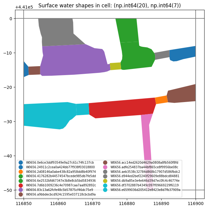
The next step is to aggregate the parameters for all the features in one grid cell to obtain one representative set of parameters. First, let’s take a look at a grid cell containing multiple features. We take the gridcell that contains the most features.

cid = sfw_grid.cellid.value_counts().index[0]
mask = sfw_grid.cellid == cid
sfw_grid.loc[mask]

	id	creationDate	LV-publicatiedatum	relatieveHoogteligging	inOnderzoek	eindRegistratie	tijdstipRegistratie	identificatie	bronhouder	bgt-status	...	terminationDate	bronhouder_name	ahn_min	summer_stage	winter_stage	geometry	stage	botm	cellid	area
559	b5a53b635-d396-a910-bd9c-46e8226ec4a4	2015-10-29	2016-07-06T15:37:15	0	false	None	2016-01-04T08:50:54.000	W0656.4176282b44574547bcede985db7fe5dd	W0656	bestaand	...	None	Hoogheemraadschap van Schieland en de Krimpene...	-1.803157	-1.91	-1.96	POLYGON ((116883.486 440993.24, 116878.898 440...	-1.935	-2.435	(20, 7)	39.950023
578	bc1e73327-d135-b9e7-e13c-17b8c4083248	2015-10-29	2016-07-06T15:37:15	0	false	None	2016-01-04T08:50:54.000	W0656.83c13a62fcfe48c5b57875cf46dc75e9	W0656	bestaand	...	None	Hoogheemraadschap van Schieland en de Krimpene...	NaN	-1.91	-1.96	POLYGON ((116873.44 440990.3, 116874.38 440986...	-1.935	-2.435	(20, 7)	156.916996
636	b277c12a5-3966-6d28-3aed-f2dd400195d7	2015-10-29	2019-08-16T18:44:11	0	false	None	2019-08-15T15:24:33.000	W0656.0e6ce3ddf93549e9a27c61c74fc137cb	W0656	bestaand	...	None	Hoogheemraadschap van Schieland en de Krimpene...	-1.149745	-1.91	-1.96	POLYGON ((116851.36 440985.97, 116851.49 44098...	-1.935	-2.435	(20, 7)	5.025221
641	bf86d3648-d739-c6cd-27fa-37eff9c50db0	2015-10-29	2019-08-16T18:44:11	0	false	None	2019-08-15T15:24:33.000	W0656.24911c2cea0a424bb77f938f03018800	W0656	bestaand	...	None	Hoogheemraadschap van Schieland en de Krimpene...	NaN	-1.91	-1.96	POLYGON ((116896.4 440988.15, 116894.52 440987...	-1.935	-2.435	(20, 7)	24.901125
649	bf005c07a-c701-61c5-bb2f-4e279861ae3b	2015-10-29	2019-08-16T18:44:11	0	false	None	2019-08-15T15:24:33.000	W0656.6e2532bfd67347e3b8e8cb5bd5834936	W0656	bestaand	...	None	Hoogheemraadschap van Schieland en de Krimpene...	-1.619307	-1.91	-1.96	POLYGON ((116883.486 440993.24, 116883.604 440...	-1.935	-2.435	(20, 7)	65.424827
652	bc9da9d09-dd92-11a5-0d43-1a2d2bb95237	2015-10-29	2019-08-16T18:44:11	0	false	None	2019-08-15T15:24:33.000	W0656.7d6b1009236c4e70987caa7aa892892c	W0656	bestaand	...	None	Hoogheemraadschap van Schieland en de Krimpene...	NaN	-1.91	-1.96	POLYGON ((116888.49 440975.04, 116887.562 4409...	-1.935	-2.435	(20, 7)	87.909658
665	be5f3176f-bdab-4958-3908-52dfc31cf0b6	2015-10-29	2019-08-16T18:44:11	0	false	None	2019-08-15T15:24:33.000	W0656.acc14ed2620d4629a0808a8fb560f8fd	W0656	bestaand	...	None	Hoogheemraadschap van Schieland en de Krimpene...	NaN	-1.91	-1.96	POLYGON ((116900 440980.894, 116900 440975.915...	-1.935	-2.435	(20, 7)	35.290249
673	b89dd3d14-6605-3507-61c7-91e2c24510a5	2015-10-29	2019-08-16T18:44:11	0	false	None	2019-08-15T15:24:33.000	W0656.d944ed2bef2240f29609e88bdcd84881	W0656	bestaand	...	None	Hoogheemraadschap van Schieland en de Krimpene...	-1.728949	-1.91	-1.96	POLYGON ((116855.33 440994.53, 116855 440995.4...	-1.935	-2.435	(20, 7)	81.433112
703	bfd6384e1-9c87-7300-1242-8ac4111813ed	2019-08-15	2019-08-16T18:44:11	0	false	None	2019-08-15T15:24:33.000	W0656.2d08146a0abe438c82a958dd8b40f974	W0656	bestaand	...	None	Hoogheemraadschap van Schieland en de Krimpene...	NaN	-1.91	-1.96	POLYGON ((116891.95 440975.57, 116888.49 44097...	-1.935	-2.435	(20, 7)	6.963900
733	b3c18517a-b046-66d5-c912-f6d5f9e438b4	2019-08-15	2019-08-16T18:44:11	0	false	None	2019-08-15T15:24:33.000	W0656.a9bbdecbcd924c1595e037118cbcbd9a	W0656	bestaand	...	None	Hoogheemraadschap van Schieland en de Krimpene...	-1.186425	-1.91	-1.96	POLYGON ((116854.79 440983.78, 116854.79 44098...	-1.935	-2.435	(20, 7)	8.207950
735	b3b28a62e-eada-92d7-c249-5b5c7bae33a7	2019-08-15	2019-08-16T18:44:11	0	false	None	2019-08-15T15:24:33.000	W0656.aeb3538c32784d868b17907d586fbdc2	W0656	bestaand	...	None	Hoogheemraadschap van Schieland en de Krimpene...	-1.376571	-1.91	-1.96	POLYGON ((116887.94 440989.98, 116892.39 44099...	-1.935	-2.435	(20, 7)	8.722850
748	b930236e9-d146-ba44-fc3a-3ec17fb6173f	2019-08-15	2019-08-16T18:44:11	0	false	None	2019-08-15T15:24:33.000	W0656.db9a85e3e4e646d39d7ec0fc4c46774e	W0656	bestaand	...	None	Hoogheemraadschap van Schieland en de Krimpene...	-1.404209	-1.91	-1.96	POLYGON ((116878.34 440985.19, 116875.24 44098...	-1.935	-2.435	(20, 7)	6.333950
751	b2a8e0641-7b6f-1650-6fce-9faa01a3d119	2019-08-15	2019-08-16T18:44:11	0	false	None	2019-08-15T15:24:33.000	W0656.df3702887b4349c097f09669229f6119	W0656	bestaand	...	None	Hoogheemraadschap van Schieland en de Krimpene...	-0.847543	-1.91	-1.96	POLYGON ((116869.078 440972.009, 116869.066 44...	-1.935	-2.435	(20, 7)	12.250377
824	b40349d0e-96cc-0253-efd2-a26f5f668705	2015-10-29	2021-04-12T14:12:16	0	false	None	2021-04-12T12:25:19.000	W0656.e6599036d205412e8423e8d7fb37909a	W0656	bestaand	...	None	Hoogheemraadschap van Schieland en de Krimpene...	-1.422086	-1.91	-1.96	POLYGON ((116864.1 440970.71, 116863.39 440970...	-1.935	-2.435	(20, 7)	102.696517
847	b60842130-ff94-9d63-daa5-457cefa454da	2021-06-07	2021-06-07T11:35:51	0	false	None	2021-06-07T11:32:43.000	W0656.adfe254837ba44bf865ce8f9956be08c	W0656	bestaand	...	None	Hoogheemraadschap van Schieland en de Krimpene...	-1.446577	-1.91	-1.96	POLYGON ((116884.286 440969.237, 116884.082 44...	-1.935	-2.435	(20, 7)	47.496899

15 rows × 23 columns

We can also plot the features within that grid cell.

fig, ax = plt.subplots(1, 1, figsize=(10, 8))
sfw_grid.loc[mask].plot(
    column="identificatie",
    legend=True,
    ax=ax,
    legend_kwds={"loc": "lower left", "ncol": 2, "fontsize": "x-small"},
)
xlim = ax.get_xlim()
ylim = ax.get_ylim()
gwf.modelgrid.plot(ax=ax)
ax.set_xlim(xlim[0], xlim[0] + nlmod.grid.get_delr(ds)[-1] * 1.1)
ax.set_ylim(ylim)
ax.set_title(f"Surface water shapes in cell: {cid}");

Now we want to aggregate the features in each cell to obtain a representative set of parameters (stage, conductance, bottom elevation) to use in the model. There are several aggregation methods. Note that the names of the methods are not representative of the aggregation applied to each parameter. For a full description see the following list:

• 'area_weighted'

  • stage: area-weighted average of stage in cell

  • cond: conductance is equal to area of surface water divided by bottom resistance

  • elev: the lowest bottom elevation is representative for the cell

• 'max_area'

  • stage: stage is determined by the largest surface water feature in a cell

  • cond: conductance is equal to area of all surface water features divided by bottom resistance

  • elev: the lowest bottom elevation is representative for the cell

• 'de_lange'

  • stage: area-weighted average of stage in cell

  • cond: conductance is calculated using the formulas derived by De Lange (1999).

  • elev: the lowest bottom elevation is representative for the cell

Let’s try using area_weighted. This means the stage is the area-weighted average of all the surface water features in a cell. The conductance is calculated by dividing the total area of surface water in a cell by the bottom resistance (c0). The representative bottom elevation is the lowest elevation present in the cell.

try:
    nlmod.gwf.surface_water.aggregate(sfw_grid, "area_weighted")
except ValueError as e:
    print(e)

Missing columns in DataFrame: {'c0'}

The function checks whether the requisite columns are defined in the DataFrame. We need to add a column containing the bottom resistance c0. Often a value of 1 day is used as an initial estimate.

sfw_grid["c0"] = 1.0  # days

Now aggregate the features.

celldata = nlmod.gwf.surface_water.aggregate(
    sfw_grid, "area_weighted", cachedir=ds.cachedir, cachename="celldata.pklz"
)

Aggregate surface water data:   0%|          | 0/3553 [00:00<?, ?it/s]
Aggregate surface water data: 100%|██████████| 3553/3553 [00:04<00:00, 771.53it/s]

Let’s take a look at the result. We now have a DataFrame with cell-id as the index and the three parameters we need for each cell stage, cond and rbot. The area is also given, but is not needed for the groundwater model.

celldata.head(10)

		stage	cond	rbot	area
0	0	-1.935	462.410287	-2.435	462.410287
	1	-1.935	459.780508	-2.435	459.780508
	2	-1.935	491.005144	-2.435	491.005144
	3	-1.935	415.290645	-2.435	415.290645
	4	-1.935	499.529157	-2.435	499.529157
	5	-1.935	412.999363	-2.435	412.999363
	6	-1.935	347.403279	-2.435	347.403279
	7	-1.935	333.055784	-2.435	333.055784
	8	-1.935	201.044358	-2.435	201.044358
	9	-1.935	427.468514	-2.435	427.468514

Build stress period data

The next step is to take our cell-data and build convert it to ‘stress period data’ for MODFLOW. This is a data format that defines the parameters in each cell in the following format:

[[(cellid1), param1a, param1b, param1c],
 [(cellid2), param2a, param2b, param2c],
 ...]

The required parameters are defined by the MODFLOW-package used:

• RIV: for the river package (stage, cond, rbot)

• DRN: for the drain package (stage, cond)

• GHB: for the general-head-boundary package (stage, cond)

We’re selecting the RIV package. We don’t have a bottom (rbot) for each reach in celldata. Therefore we remove the reaches where rbot is nan (not a number).

new_celldata = celldata.loc[~celldata.rbot.isna()]
print(f"removed {len(celldata)-len(new_celldata)} reaches because rbot is nan")

removed 57 reaches because rbot is nan

riv_spd = nlmod.gwf.surface_water.build_spd(new_celldata, "RIV", ds)

Building stress period data RIV:   0%|          | 0/3496 [00:00<?, ?it/s]
Building stress period data RIV: 100%|██████████| 3496/3496 [00:00<00:00, 5650.10it/s]

Take a look at the stress period data for the river package:

riv_spd[:10]

[[(np.int64(0), 0, 0),
  np.float64(-1.935),
  np.float64(462.4102867442484),
  np.float64(-2.435)],
 [(np.int64(0), 0, 1),
  np.float64(-1.9349999999999998),
  np.float64(459.780507649758),
  np.float64(-2.435)],
 [(np.int64(0), 0, 2),
  np.float64(-1.9350000000000003),
  np.float64(491.00514351109155),
  np.float64(-2.435)],
 [(np.int64(0), 0, 3),
  np.float64(-1.9349999999999996),
  np.float64(415.2906454126869),
  np.float64(-2.435)],
 [(np.int64(0), 0, 4),
  np.float64(-1.9350000000000003),
  np.float64(499.52915726560855),
  np.float64(-2.435)],
 [(np.int64(0), 0, 5),
  np.float64(-1.935),
  np.float64(412.99936270143803),
  np.float64(-2.435)],
 [(np.int64(0), 0, 6),
  np.float64(-1.935),
  np.float64(347.4032788950671),
  np.float64(-2.435)],
 [(np.int64(0), 0, 7),
  np.float64(-1.935),
  np.float64(333.05578372039884),
  np.float64(-2.435)],
 [(np.int64(0), 0, 8),
  np.float64(-1.9349999999999998),
  np.float64(201.04435784327512),
  np.float64(-2.435)],
 [(np.int64(0), 0, 9),
  np.float64(-1.9350000000000003),
  np.float64(427.4685140175443),
  np.float64(-2.435)]]

Create RIV package

The final step is to create the river package using flopy.

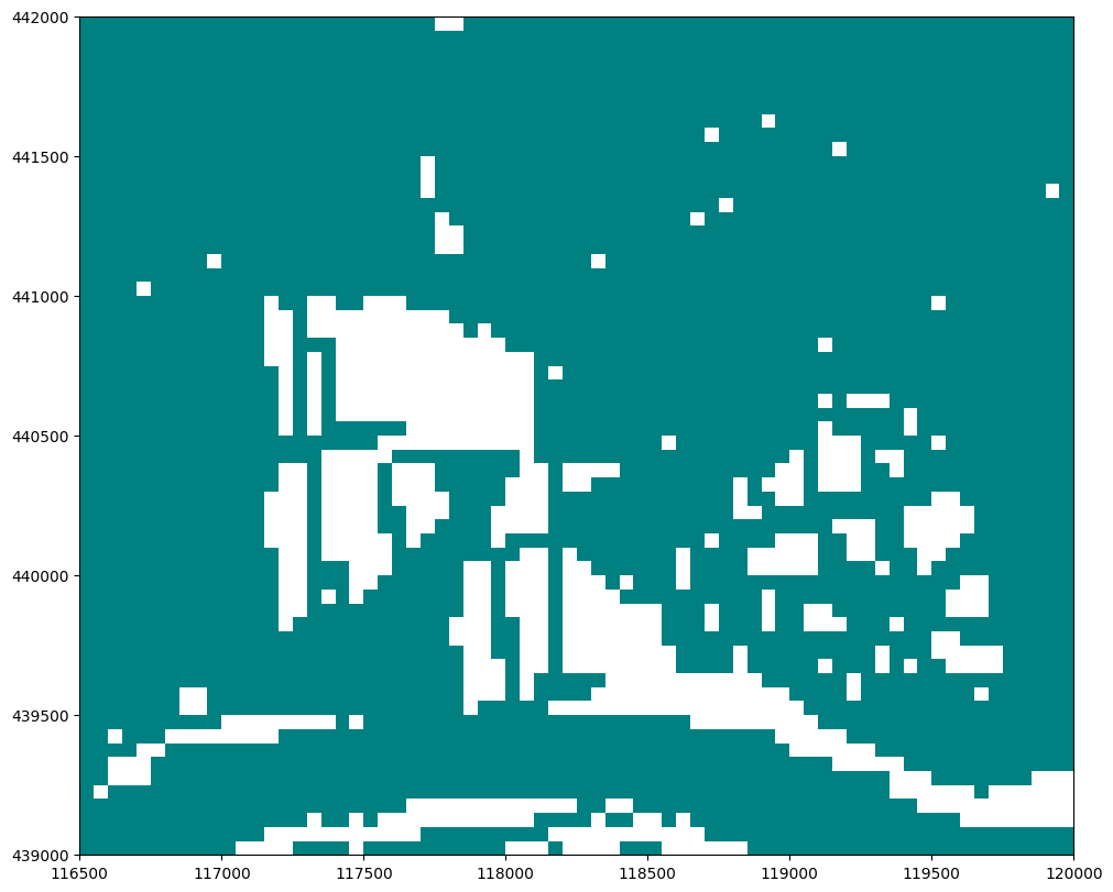
riv = flopy.mf6.ModflowGwfriv(gwf, stress_period_data=riv_spd)

Plot the river boundary condition to see where rivers were added in the model

# use flopy plotting methods
fig, ax = plt.subplots(1, 1, figsize=(10, 8), constrained_layout=True)
mv = flopy.plot.PlotMapView(model=gwf, ax=ax, layer=0)
mv.plot_bc("RIV")

<matplotlib.collections.QuadMesh at 0x73d21a5360d0>

Write + run model

Now write the model simulation to disk, and run the simulation.

nlmod.sim.write_and_run(sim, ds, write_ds=True)

writing simulation...
  writing simulation name file...
  writing simulation tdis package...
  writing solution package ims...
  writing model Schoonhoven...
    writing model name file...
    writing package dis...
    writing package npf...
    writing package ic...
    writing package oc...
    writing package riv_0...
INFORMATION: maxbound in ('', 'riv', 'dimensions') changed to 3496 based on size of stress_period_data
FloPy is using the following executable to run the model: ../../../../../envs/latest/lib/python3.11/site-packages/nlmod/bin/mf6
                                   MODFLOW 6
                U.S. GEOLOGICAL SURVEY MODULAR HYDROLOGIC MODEL
                            VERSION 6.6.3 09/29/2025

   MODFLOW 6 compiled Oct 07 2025 22:51:46 with Intel(R) Fortran Intel(R) 64
   Compiler Classic for applications running on Intel(R) 64, Version 2021.7.0
                             Build 20220726_000000

This software has been approved for release by the U.S. Geological 
Survey (USGS). Although the software has been subjected to rigorous 
review, the USGS reserves the right to update the software as needed 
pursuant to further analysis and review. No warranty, expressed or 
implied, is made by the USGS or the U.S. Government as to the 
functionality of the software and related material nor shall the 
fact of release constitute any such warranty. Furthermore, the 
software is released on condition that neither the USGS nor the U.S. 
Government shall be held liable for any damages resulting from its 
authorized or unauthorized use. Also refer to the USGS Water 
Resources Software User Rights Notice for complete use, copyright, 
and distribution information.

 
 MODFLOW runs in SEQUENTIAL mode
 
 Run start date and time (yyyy/mm/dd hh:mm:ss): 2026/05/13 15:16:40
 
 Writing simulation list file: mfsim.lst
 Using Simulation name file: mfsim.nam
    Solving:  Stress period:     1    Time step:     1
 
 Run end date and time (yyyy/mm/dd hh:mm:ss): 2026/05/13 15:16:40
 Elapsed run time:  0.670 Seconds
 
 Normal termination of simulation.

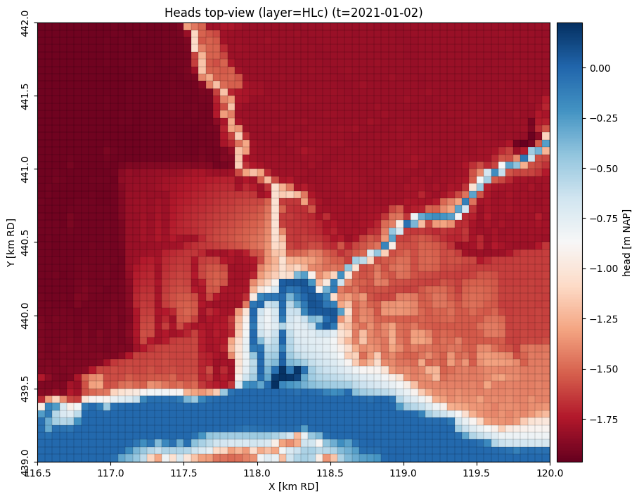
Visualize results

To see whether our surface water was correctly added to the model, let’s visualize the results. We’ll load the calculated heads, and plot them.

head = nlmod.gwf.get_heads_da(ds)

Plot the heads in a specific model layer

# using nlmod plotting methods
ax = nlmod.plot.map_array(
    head,
    ds,
    ilay=0,
    iper=0,
    plot_grid=True,
    title="Heads top-view",
    cmap="RdBu",
    colorbar_label="head [m NAP]",
)

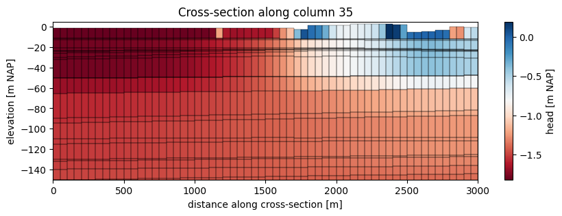
In cross-section

# using flopy plotting methods
col = gwf.modelgrid.ncol // 2

fig, ax = plt.subplots(1, 1, figsize=(10, 3))
xs = flopy.plot.PlotCrossSection(model=gwf, ax=ax, line={"column": col})
qm = xs.plot_array(head[-1], cmap="RdBu")  # last timestep
xs.plot_ibound()  # plot inactive cells in red
xs.plot_grid(lw=0.25, color="k")
ax.set_ylim(bottom=-150)
ax.set_ylabel("elevation [m NAP]")
ax.set_xlabel("distance along cross-section [m]")
ax.set_title(f"Cross-section along column {col}")
cbar = fig.colorbar(qm, shrink=1.0)
cbar.set_label("head [m NAP]")