Stromingen example: keeping scripts simple

This example is based on the essay “Open source grondwatermodellering met MODFLOW 6” that was published in Stromingen (Calje et al., 2022).

This example strives to achieve the simplicity of the example psuedo script that was shown in Figure 5 in the article. Some things require a bit more code than in the example, but not by much! Also some data is not yet publicly accessible, i.e. well data, so that has also not yet been implemented in this example. We also changed the extent to build a smaller model (because of computation time).

Import Python packages

import os

import flopy as fp
import geopandas as gpd
from pandas import date_range

import nlmod

nlmod.util.get_color_logger("INFO")
nlmod.show_versions()

Python version     : 3.11.14
NumPy version      : 2.4.4
Xarray version     : 2026.4.0
Matplotlib version : 3.10.9
Flopy version      : 3.10.0

nlmod version      : 0.11.3dev

Define spatial and temporal properties

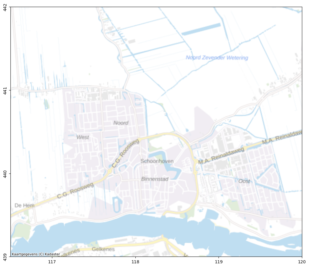
extent = [116_500, 120_000, 439_000, 442_000]
tmin = "2010-01-01"
tmax = "2020-01-01"
freq = "14D"

# where in the world are we?
nlmod.plot.get_map(extent, background=True);

Get data for the current extent

# define a model workspace for caching downloaded data
model_ws = "14_stromingen_example"
figdir, cachedir = nlmod.util.get_model_dirs(model_ws)

layer_model = nlmod.read.regis.get_combined_layer_models(
    extent,
    use_regis=True,
    use_geotop=False,
    cachedir=cachedir,
    cachename="layer_model.nc",
)

# wells = nlmod.read.get_wells(extent)  # no well data is available just yet

# surface water features and levels
fname_bgt = os.path.join("..", "data_sources", "02_surface_water", "cache", "bgt.gpkg")
if not os.path.isfile(fname_bgt):
    raise (
        Exception(
            f"{fname_bgt} not found. Please run notebook 02_surface_water.ipynb first"
        )
    )
sw = gpd.read_file(fname_bgt)

WARNING:nlmod.dims.layers.remove_layer_dim_from_top:Botm of layer is not equal to top of deeper layer in 3 cells
INFO:nlmod.cache.wrapper:caching data -> layer_model.nc

Generate grid with a refinement zone

# create a model dataset
ds = nlmod.to_model_ds(layer_model, "stromingen", model_ws=model_ws)

# refine model dataset (supply a list of xy-coordinates)
xy = [
    [
        [
            (117_500, 439_500),
            (117_500, 440_000),
            (118_000, 440_000),
            (118_000, 439_500),
            (117_500, 439_500),
        ]
    ]
]

refinement = [(xy, "polygon", 1)]
ds = nlmod.grid.refine(ds, refinement_features=refinement)

INFO:nlmod.dims.base.to_model_ds:resample layer model data to structured modelgrid
INFO:nlmod.dims.layers.get_kh_kv:kv and kh both undefined in layer HLc
INFO:nlmod.dims.layers._fill_var:Filling 7594 values in active cells of kh by multipying kv with an anisotropy of 10
INFO:nlmod.dims.layers._fill_var:Filling 16762 values in active cells of kv by dividing kh by an anisotropy of 10
INFO:nlmod.dims.layers._fill_var:Filling 1050 values in active cells of kh with a value of 1.0 m/day
INFO:nlmod.dims.layers._fill_var:Filling 1050 values in active cells of kv with a value of 0.1 m/day
INFO:nlmod.dims.grid.refine:create vertex grid using gridgen
INFO:nlmod.dims.grid.ds_to_gridprops:resample model Dataset to vertex modelgrid

Generate a model

# set model time settings
t = date_range(tmin, tmax, freq=freq)
ds = nlmod.time.set_ds_time(ds, start=3652, time=t, steady_start=True)

# build the modflow6 gwf model
gwf = nlmod.gwf.ds_to_gwf(ds)

INFO:nlmod.sim.sim.sim:creating mf6 SIM
INFO:nlmod.sim.sim.tdis:creating mf6 TDIS
INFO:nlmod.sim.sim.ims:creating mf6 IMS
INFO:nlmod.gwf.gwf.gwf:creating mf6 GWF
INFO:nlmod.gwf.gwf._disv:creating mf6 DISV
INFO:nlmod.gwf.gwf.npf:creating mf6 NPF
INFO:nlmod.gwf.gwf.ic:creating mf6 IC
INFO:nlmod.gwf.gwf.ic:adding 'starting_head' data array to ds
INFO:nlmod.gwf.gwf.oc:creating mf6 OC

Add recharge to the model

# download knmi recharge data
knmi_ds = nlmod.read.knmi.get_recharge(ds)

# update model dataset
ds.update(knmi_ds)

# create recharge package
rch = nlmod.gwf.rch(ds, gwf)

INFO:hydropandas.io.knmi.get_knmi_obs:get data from station 434 and variable RD from 2000-01-02 to 2019-12-20
INFO:hydropandas.io.knmi.get_knmi_obs:get data from station 348 and variable EV24 from 2000-01-02 to 2019-12-20
WARNING:nlmod.read.knmi.discretize_knmi:The default of hourly_precision=False will be changed to True in a future version of nlmod. Pass hourly_precision=False to retain current behavior or hourly_precision=True to adopt the future default and silence this warning.
INFO:nlmod.gwf.gwf.rch:creating mf6 RCH

Add surface water to the model

# set stage for model to mean of summer and winter levels
sw["stage"] = sw[["winter_stage", "summer_stage"]].mean(axis=1)

# use a water depth of 0.5 meter
sw["rbot"] = sw["stage"] - 0.5

# set the stage of the Lek river to 0.0 m NAP and the botm to -3 m NAP
mask = sw["bronhouder"] == "L0002"
sw.loc[mask, "stage"] = 0.0
sw.loc[mask, "rbot"] = -3.0

# we need to mask out the NaNs
sw.drop(sw.index[sw["rbot"].isna()], inplace=True)

# intersect surface water with grid
sfw_grid = nlmod.grid.gdf_to_grid(sw, gwf)

# add bed resistance to calculate conductance
bed_resistance = 1.0  # days
sfw_grid["cond"] = sfw_grid.area / bed_resistance
sfw_grid.set_index("cellid", inplace=True)

# build stress period data for RIV package
riv_spd = nlmod.gwf.surface_water.build_spd(sfw_grid, "RIV", ds)

Intersecting with grid:   0%|          | 0/1460 [00:00<?, ?it/s]
Intersecting with grid: 100%|██████████| 1460/1460 [00:05<00:00, 279.94it/s]
Building stress period data RIV:   0%|          | 0/4313 [00:00<?, ?it/s]
Building stress period data RIV: 100%|██████████| 4313/4313 [00:00<00:00, 7914.20it/s]

# flopy is used to construct the RIV package directly
riv = fp.mf6.ModflowGwfriv(gwf, stress_period_data=riv_spd)

Run model

nlmod.sim.write_and_run(gwf, ds, silent=True)

INFO:nlmod.sim.sim.write_and_run:write model dataset to cache
INFO:nlmod.sim.sim.write_and_run:write modflow files to model workspace
INFO:nlmod.sim.sim.write_and_run:run model

Post-processing

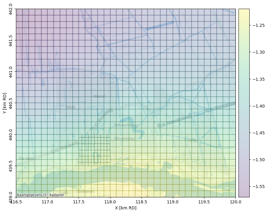
Plotting the average head in REGIS layer PZWAz3

# load the computed heads
head = nlmod.gwf.output.get_heads_da(ds)

# plot on map
ax = nlmod.plot.map_array(
    head.sel(layer="PZWAz3").mean(dim="time"),
    ds,
    alpha=0.25,
    background=True,
)

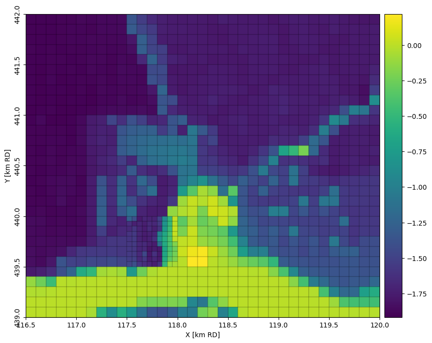
Plot the GHG in the upper layer, named ‘HLc’.

# use nlmod's calculate_gxg method to calculate the GVG, GLG and GHG.
gxg = nlmod.gwf.calculate_gxg(head.sel(layer="HLc"))

# plot on map
pc = nlmod.plot.map_array(gxg["ghg"], ds)

References

• Calje, R., F. Schaars, D. Brakenhoff, O. Ebbens. (2022) “Open source grondwatermodellering met MODFLOW 6”. Stromingen 2022 Vol. 03.