Downloading surface water data

This section notebook shows some how to download surface water data into a GeoDataFrame using the nlmod package.

We select an area near around Schoonhoven for this demonstration. There are three water boards in the this area, and we download seasonal data about the stage of the surface water for each. For locations without a stage from the water board, we obtain information from a Digital Terrain Model near the surface water features, to estimate a stage. We assign a stage of 0.0 m NAP to the river Lek.

import os
import rioxarray
import nlmod

nlmod.util.get_color_logger("INFO")
nlmod.show_versions()

Python version     : 3.11.14
NumPy version      : 2.4.4
Xarray version     : 2026.4.0
Matplotlib version : 3.10.9
Flopy version      : 3.10.0

nlmod version      : 0.11.3dev

First we specify a folder where we can save downloaded data to and define the extent of our model.

model_name = "steady"
model_ws = "02_surface_water"
figdir, cachedir = nlmod.util.get_model_dirs(model_ws)
extent = [116_500, 120_000, 439_000, 442_000]

AHN

Download the Digital Terrain model of the Netherlands (AHN). To speed up this notebook we download data on a resolution of 5 meter. We can change this to a resolution of 0.5 meter, changing the identifier to “AHN4_DTM_05m”.

fname_ahn = os.path.join(cachedir, "ahn.tif")
if not os.path.isfile(fname_ahn):
    ahn = nlmod.read.ahn.download_ahn4(extent)
    ahn.rio.to_raster(fname_ahn)
ahn = rioxarray.open_rasterio(fname_ahn, mask_and_scale=True)[0]

Downloading tiles of AHN4:   0%|          | 0/1 [00:00<?, ?it/s]
Downloading tiles of AHN4: 100%|██████████| 1/1 [00:03<00:00,  3.63s/it]

Layer ‘waterdeel’ from bgt

As the source of the location of the surface water bodies we use the ‘waterdeel’ layer of the Basisregistratie Grootschalige Topografie (BGT). This data consists of detailed polygons, maintained by dutch government agencies (water boards, municipalities and Rijkswaterstaat).

bgt = nlmod.read.bgt.download_bgt(extent)

Add minimum surface height around surface water bodies

Get the minimum surface level in 5 meter around surface water levels and add these data to the column ‘ahn_min’.

bgt = nlmod.gwf.add_min_ahn_to_gdf(bgt, ahn, buffer=5.0, column="ahn_min")

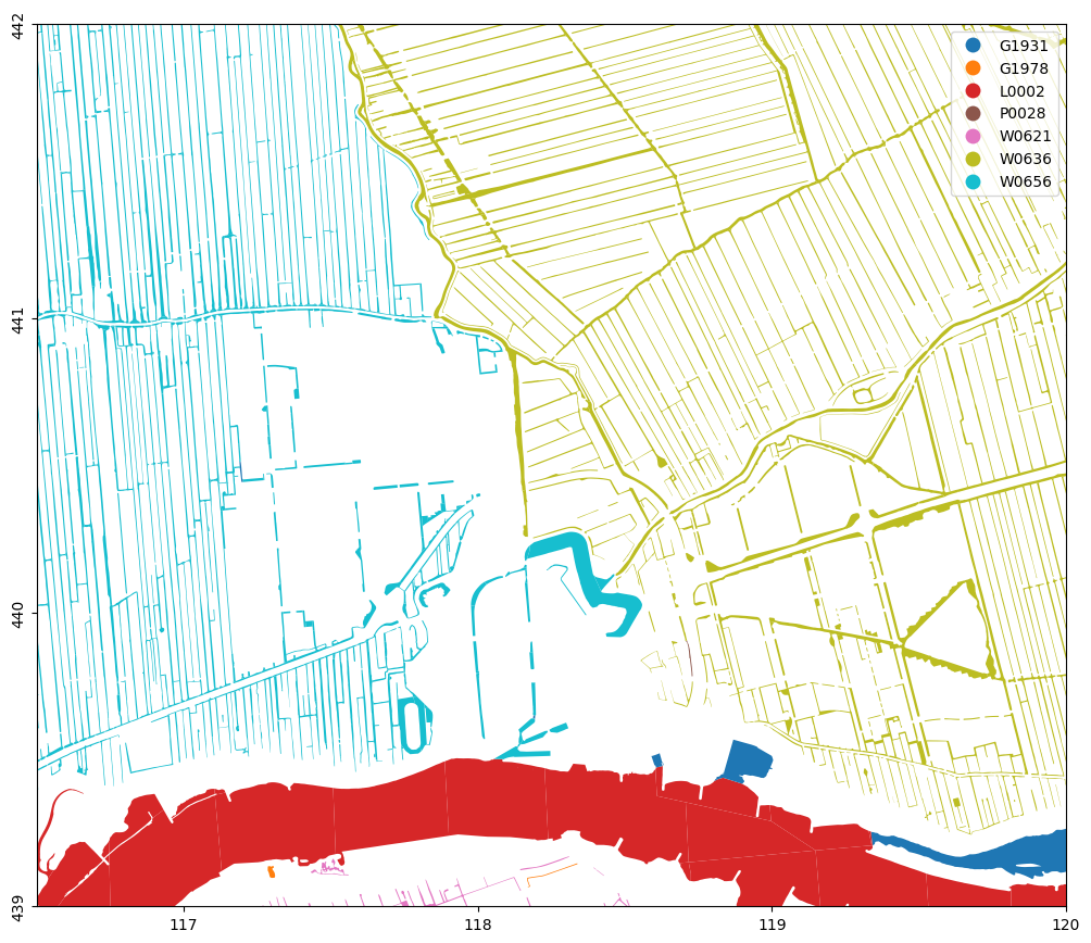
Plot ‘bronhouder’

We can plot the column ‘bronhouder’ from the GeoDataFrame bgt. We see there are three water boards in this area (with codes starting with ‘W’).

f, ax = nlmod.plot.get_map(extent)
bgt.plot("bronhouder", legend=True, ax=ax)

<Axes: >

level areas

For these three waterboards we download the level areas (peilgebieden): polygons with information about winter and summer stages.

la = nlmod.gwf.surface_water.download_level_areas(
    bgt, extent=extent, raise_exceptions=False
)

INFO:nlmod.gwf.surface_water.download_level_areas:Downloading level_areas for De Stichtse Rijnlanden
INFO:nlmod.gwf.surface_water.download_level_areas:Downloading level_areas for Rivierenland
INFO:nlmod.gwf.surface_water.download_level_areas:Downloading level_areas for Schieland en de Krimpenerwaard

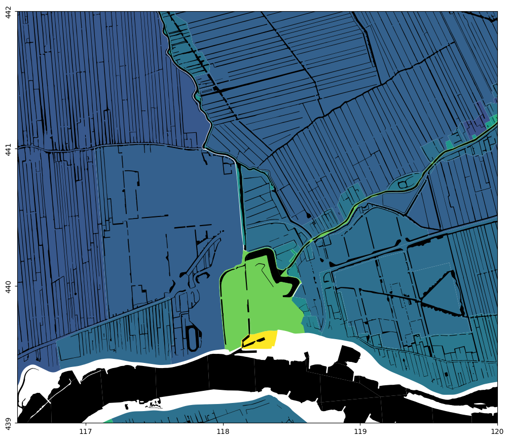
Plot summer stage

The method download_level_areas() generates a dictionary with the name of the water boards as keys and GeoDataFrames as values. Each GeoDataFrame contains the columns summer_stage and winter_stage. Let’s plot the summer stage, together with the location of the surface water bodies.

f, ax = nlmod.plot.get_map(extent)
bgt.plot(color="k", ax=ax)
for wb in la:
    la[wb].plot("summer_stage", ax=ax, vmin=-3, vmax=1, zorder=0)

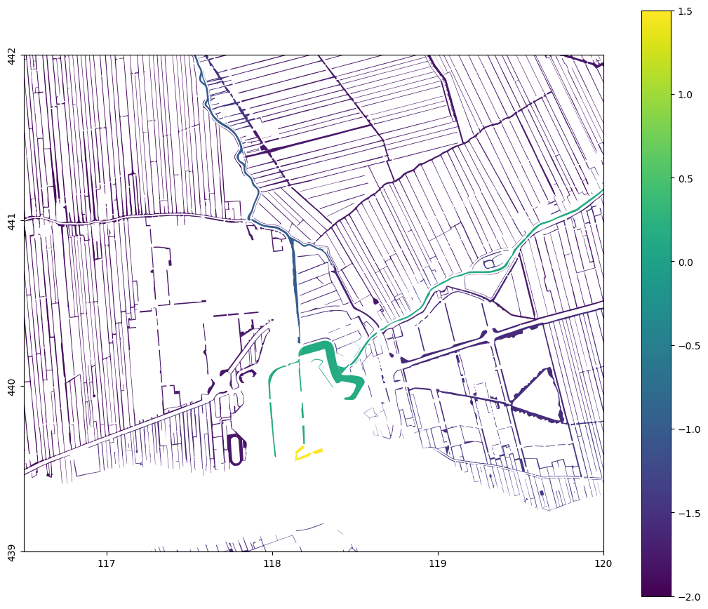
Add stages to bgt-data

We then add the information from these level areas to the surface water bodies. Afterwards we can then again plot the summer-stage, but now for the individual water bodies.

bgt = nlmod.gwf.surface_water.add_stages_from_waterboards(bgt, la=la)
fig, ax = nlmod.plot.get_map(extent)
bgt.plot(ax=ax, column="summer_stage", legend=True);

Adding ['summer_stage', 'winter_stage'] from De Stichtse Rijnlanden:   0%|          | 0/542 [00:00<?, ?it/s]
Adding ['summer_stage', 'winter_stage'] from De Stichtse Rijnlanden: 100%|██████████| 542/542 [00:00<00:00, 733.12it/s]
Adding ['summer_stage', 'winter_stage'] from Rivierenland:   0%|          | 0/21 [00:00<?, ?it/s]
Adding ['summer_stage', 'winter_stage'] from Rivierenland: 100%|██████████| 21/21 [00:00<00:00, 934.23it/s]
Adding ['summer_stage', 'winter_stage'] from Schieland en de Krimpenerwaard:   0%|          | 0/875 [00:00<?, ?it/s]
Adding ['summer_stage', 'winter_stage'] from Schieland en de Krimpenerwaard: 100%|██████████| 875/875 [00:01<00:00, 862.18it/s]

Save the data to use in other notebooks as well

We save the bgt-data to a GeoPackage file, so we can use the data in other notebooks with surface water as well.

fname_bgt = os.path.join(cachedir, "bgt.gpkg")
bgt.to_file(fname_bgt)

INFO:pyogrio._io.write:Created 1,470 records