Unsaturated Zone Flow

This notebook demonstrates the use of the Unsaturated Zone Flow (UZF) package in nlmod. The UZF-package can be used to simulate important processes in the unsaturated zone. These processes create a delay before precipitation reaches the saturated groundwater. In dry periods the water may even have evaporated before that. This notebook shows the difference in calculated head between a model with regular recharge (RCH) and evapotranspiration (EVT) packages, compared to a model with the UZF-package.

We create a 1d model, consisting of 1 row and 1 column with multiple layers, of a real location somewhere in the Netherlands. We use weather data from the KNMI as input for a transient simulation of 3 years with daily timetseps. This notebook can be used to vary the uzf-parameters, change the location (do not forget to alter the drain-elevation as well), or to play with the model timestep.

Import packages and setup logging

# import packages
import os

import matplotlib.pyplot as plt
import numpy as np
import pandas as pd

import nlmod

# set up pretty logging and show package versions
nlmod.util.get_color_logger()
nlmod.show_versions()

Python version     : 3.11.14
NumPy version      : 2.4.4
Xarray version     : 2026.4.0
Matplotlib version : 3.10.9
Flopy version      : 3.10.0

nlmod version      : 0.11.3dev

Generate a model Dataset

We first set the model_name and model workspace, which we will use later to write the model files, and so we can determine the cache-directory.

model_name = "model17"
model_ws = "17_unsaturated_zone_flow"
figdir, cachedir = nlmod.util.get_model_dirs(model_ws)

We define a location with a corresponding drainage elevation. From the location we calculate an extent of 100 by 100 meter, and download REGIS.

x = 37_400
y = 412_600
drn_elev = 4.0

# round x and y to 100, so we will download only one cell in regis
x = np.floor(x / 100) * 100
y = np.floor(y / 100) * 100
dx = dy = 100
extent = [x, x + dx, y, y + dy]
regis = nlmod.read.regis.download_regis(
    extent, drop_layer_dim_from_top=False, cachename="regis.nc", cachedir=cachedir
)

INFO:nlmod.cache.wrapper:caching data -> regis.nc

As the REGIS-data only contains one cell, we can visualize the properties of the layers in a pandas DataFrame.

regis.sel(x=regis.x[0], y=regis.y[0]).to_pandas()

	top	botm	kh	kv	x	y	spatial_ref
layer
HLc	6.490000	-14.530000	NaN	NaN	37450.0	412650.0	0
BXz2	-14.530000	-17.309999	4.06	NaN	37450.0	412650.0	0
BXz3	-17.309999	-18.070000	4.06	NaN	37450.0	412650.0	0
BXz4	-18.070000	-26.920000	4.13	NaN	37450.0	412650.0	0
EEz1	-26.920000	-29.770000	12.26	NaN	37450.0	412650.0	0
EEz2	-29.770000	-31.680000	12.40	NaN	37450.0	412650.0	0
EEz3	-31.680000	-43.580002	12.53	NaN	37450.0	412650.0	0
PZWAz2	-43.580002	-43.680000	8.85	NaN	37450.0	412650.0	0
PZWAz3	-43.680000	-45.040001	7.80	NaN	37450.0	412650.0	0
PZWAz4	-45.040001	-46.500000	6.62	NaN	37450.0	412650.0	0
MSk1	-46.500000	-50.279999	NaN	0.004486	37450.0	412650.0	0
MSz2	-50.279999	-59.459999	6.27	NaN	37450.0	412650.0	0
MSz3	-59.459999	-77.879997	5.25	NaN	37450.0	412650.0	0
OOz1	-77.879997	-83.209999	6.76	NaN	37450.0	412650.0	0
OOk1	-83.209999	-90.220001	NaN	0.005853	37450.0	412650.0	0
OOz2	-90.220001	-108.870003	12.80	NaN	37450.0	412650.0	0
BRz1	-108.870003	-129.250000	3.66	NaN	37450.0	412650.0	0

As you can see, there are some NaN-values in the hydaulic conductivities (kh and kv). These will be filled when making a model Dataset, using fill-values and anisotropy values. See the info-messages after the commands below.

ds = nlmod.to_model_ds(
    regis,
    model_name=model_name,
    model_ws=model_ws,
    fill_value_kh=10.0,
    fill_value_kv=10.0,
)

INFO:nlmod.dims.base.to_model_ds:resample layer model data to structured modelgrid
INFO:nlmod.dims.layers.get_kh_kv:kv and kh both undefined in layer HLc
INFO:nlmod.dims.layers._fill_var:Filling 2 values in active cells of kh by multipying kv with an anisotropy of 10
INFO:nlmod.dims.layers._fill_var:Filling 14 values in active cells of kv by dividing kh by an anisotropy of 10
INFO:nlmod.dims.layers._fill_var:Filling 1 values in active cells of kh with a value of 10.0 m/day
INFO:nlmod.dims.layers._fill_var:Filling 1 values in active cells of kv with a value of 10.0 m/day

We then add a time-dimension to our model Dataset and download knmi-data. We will have a calculation period of 3 year with daily timesteps, with a steady-state stress period with the weather of 2019 as a warmup period.

time = pd.date_range("2020", "2023", freq="D")
ds = nlmod.time.set_ds_time(ds, start="2019", time=time, steady_start=True)

ds.update(
    nlmod.read.knmi.get_recharge(
        ds, method="separate", cachename="recharge.nc", cachedir=ds.cachedir
    )
)

INFO:hydropandas.io.knmi.get_knmi_obs:get data from station 734 and variable RD from 2019-01-01 to 2023-01-01
INFO:hydropandas.io.knmi.fill_missing_measurements:station 734 has no measurements between 2019-01-01 00:00:00 and 2023-01-01 00:00:00 trying to get measurements from nearest station -> 752
INFO:hydropandas.io.knmi.get_knmi_obs:get data from station 323 and variable EV24 from 2019-01-01 to 2023-01-01
INFO:hydropandas.io.knmi.fill_missing_measurements:Filled 4 observations from station 310 VLISSINGEN -> 323 WILHELMINADORP
WARNING:nlmod.read.knmi.discretize_knmi:The default of hourly_precision=False will be changed to True in a future version of nlmod. Pass hourly_precision=False to retain current behavior or hourly_precision=True to adopt the future default and silence this warning.
INFO:nlmod.cache.wrapper:caching data -> recharge.nc

Generate a simulation (sim) and groundwater flow (gwf) object

We generate a model using with all basic packages. We add a drainage level at 4.0 m NAP. As the top of our model is at 6.5 m NAP this will create an unsaturated zone of about 2.5 m.

# create simulation
sim = nlmod.sim.sim(ds)

# create time discretisation
_ = nlmod.sim.tdis(ds, sim)

# create groundwater flow model
gwf = nlmod.gwf.gwf(ds, sim, under_relaxation=True)

# create ims
_ = nlmod.sim.ims(sim)

# Create discretization
_ = nlmod.gwf.dis(ds, gwf)

# create node property flow
_ = nlmod.gwf.npf(ds, gwf, icelltype=1)

# creat storage
_ = nlmod.gwf.sto(ds, gwf, iconvert=1, sy=0.2, ss=1e-5)

# Create the initial conditions package
_ = nlmod.gwf.ic(ds, gwf, starting_head=1.0)

# Create the output control package
_ = nlmod.gwf.oc(ds, gwf)

# set a drainage level with a resistance of 100 days in the layer that contains the drainage level
cond = ds["area"] / 100.0
layer = nlmod.layers.get_layer_of_z(ds, drn_elev)
_ = nlmod.gwf.drn(ds, gwf, elev=drn_elev, cond=cond, layer=layer)

INFO:nlmod.sim.sim.sim:creating mf6 SIM
INFO:nlmod.sim.sim.tdis:creating mf6 TDIS
INFO:nlmod.gwf.gwf.gwf:creating mf6 GWF
INFO:nlmod.sim.sim.ims:creating mf6 IMS
INFO:nlmod.gwf.gwf._dis:creating mf6 DIS
INFO:nlmod.gwf.gwf.npf:creating mf6 NPF
INFO:nlmod.gwf.gwf.sto:creating mf6 STO
INFO:nlmod.gwf.gwf.ic:creating mf6 IC
INFO:nlmod.gwf.gwf.ic:adding 'starting_head' data array to ds
INFO:nlmod.gwf.gwf.oc:creating mf6 OC
INFO:nlmod.gwf.gwf.drn:creating mf6 DRN
INFO:nlmod.util._get_value_from_ds_datavar:Using user-provided 'cond' and not stored data variable 'ds.area'

Run model with RCH and EVT packages

We first run the model with the Recharge (RCH) and Evapotranspiration (EVT) packages, as a reference for the model with the UZF-package.

# create recharge package
nlmod.gwf.rch(ds, gwf)

# create evapotranspiration package
nlmod.gwf.evt(ds, gwf);

INFO:nlmod.gwf.gwf.rch:creating mf6 RCH
INFO:nlmod.gwf.gwf.evt:creating mf6 EVT
INFO:nlmod.gwf.recharge.ds_to_evt:Setting evaporation surface to 1 meter below top
INFO:nlmod.gwf.recharge.ds_to_evt:Setting extinction depth to 1 meter below surface

We run this model, read the heads and get the groundwater level (the head in the highest active cell). We save the groundwater level to a variable called gwl_rch_evt, which we will plot later on.

# run model
nlmod.sim.write_and_run(sim, ds, silent=True)

# get heads
head_rch = nlmod.gwf.get_heads_da(ds)

# calculate groundwater level
gwl_rch_evt = nlmod.gwf.output.get_gwl_from_wet_cells(head_rch, botm=ds["botm"])

INFO:nlmod.sim.sim.write_and_run:write model dataset to cache
INFO:nlmod.sim.sim.write_and_run:write modflow files to model workspace
INFO:nlmod.sim.sim.write_and_run:run model

Run model with UZF package

We then run the model again with the uzf-package. Before creating the uzf-package we remove the RCH- and EVT-packages.

We choose some values for the residual water content, the saturated water content and the exponent used in the Brooks-Corey function. Other parameters are left to their defaults. The method nlmod.gwf.uzf will generate the UZF-package, using the variable kv from ds for the saturated vertical hydraulic conductivity, the variable recharge from ds for the infiltration rate and the variable evaporation from ds as the potential evapotranspiration rate.

There can be multiple layers in the unsaturated zone, just like in the saturated zone. The method nlmod.gwf.uzf connects the unsaturated zone cells above each other.

Because we want to plot the water content in the subsurface we will add some observations of the water content to the uzf-package. We do this by adding the optional parameter obs_z to nlmod.gwf.uzf. This will create the observations in the corresponding uzf-cells, at the requested z-values (in m NAP).

gwf.remove_package("RCH")
gwf.remove_package("EVT")

# create uzf package
thtr = 0.1  # residual (irreducible) water content
thts = 0.3  # saturated water content
eps = 3.5  # exponent used in the Brooks-Corey function
# add observations of the water concent every 0.2 m, from 1 meter below the drainage-elevation to the model top
obs_z = np.arange(drn_elev - 1, ds["top"].max(), 0.2)[::-1]
_ = nlmod.gwf.uzf(
    ds,
    gwf,
    thtr=thtr,
    thts=thts,
    thti=thtr,
    eps=eps,
    print_input=True,
    print_flows=True,
    nwavesets=100,  # Modflow 6 failed and advised to increase this value from the default value of 40
    obs_z=obs_z,
)

INFO:nlmod.gwf.gwf.uzf:creating mf6 UZF
INFO:nlmod.gwf.recharge.ds_to_uzf:Setting extinction depth (extdp) to 2.0 meter below top

We run the model again, and save the groundwater level to a variable called gwl_uzf.

# run model
nlmod.sim.write_and_run(sim, ds, silent=True)

# get heads
head_rch = nlmod.gwf.get_heads_da(ds)

# calculate groundwater level
gwl_uzf = nlmod.gwf.output.get_gwl_from_wet_cells(head_rch, botm=ds["botm"])

INFO:nlmod.sim.sim.write_and_run:write model dataset to cache
INFO:nlmod.sim.sim.write_and_run:write modflow files to model workspace
INFO:nlmod.sim.sim.write_and_run:run model

We read the water content from the observations, and use the name of the observations to determine the layer, row, columns and z-value of each observation, which we can use in our plot.

# %%
fname = os.path.join(ds.model_ws, f"{ds.model_name}.uzf.obs.csv")
obs = pd.read_csv(fname, index_col=0)
obs.index = pd.to_datetime(ds.time.start) + pd.to_timedelta(obs.index, "D")
kind, lay, row, col, z = zip(*[x.split("_") for x in obs.columns])
lays = np.array([int(x) for x in lay])
rows = np.array([int(x) for x in row])
cols = np.array([int(x) for x in col])
z = np.array([float(x) for x in z])

Compare models

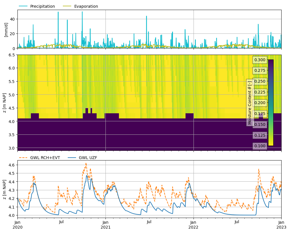
We then make a plot to compare the heads in the two simulations we performed, and plot the water content we calculated in the UZF-calculation, and added observations for. We plot the water content in one vertical cell of the model. Figure layout thanks to Martin Vonk!

The figure shows that the effect of precipitation on the groundwater level is less in summer if we also take the effect of the unsaturated zone into account (using UZF). In dry periods precipitation never reaches the groundwater level, as evaporation takes place before that.

row = 0
col = 0

f, ax = plt.subplot_mosaic(
    [["P"], ["WC"], ["H"]], figsize=(10, 8), height_ratios=[2, 5, 3], sharex=True, layout="constrained"
)

# top ax
p = ds["recharge"][:, row, col].to_pandas() * 1e3
p.plot(ax=ax["P"], label="Precipitation", color="C9")
e = ds["evaporation"][:, row, col].to_pandas() * 1e3
e.plot(ax=ax["P"], label="Evaporation", color="C8")
ax["P"].set_ylabel("[mm/d]")
ax["P"].set_ylim(bottom=0)
ax["P"].legend(loc=(0, 1), ncol=2, frameon=False)
ax["P"].grid()

# middle ax
mask = (rows == row) & (cols == col)
XY = np.meshgrid(obs.index, z[mask])
theta = obs.loc[:, mask].transpose().values
pcm = ax["WC"].pcolormesh(XY[0], XY[1], theta, cmap="viridis_r", vmin=thtr, vmax=thts)
ax["WC"].set_ylabel("z [m NAP]")
ax["WC"].grid()
# set xlim, as pcolormesh increases xlim a bit
ax["WC"].set_xlim(ds.time[0], ds.time[-1])
nlmod.plot.colorbar_inside(pcm, ax=ax["WC"], label=r"Moisture Content $\theta$ [-]")

# bottom ax
s = gwl_rch_evt[:, row, col].to_pandas()
ax["H"].plot(s.index, s.values, color="C1", linestyle="--", label="GWL RCH+EVT")
s = gwl_uzf[:, row, col].to_pandas()
ax["H"].plot(s.index, s.values, color="C0", linestyle="-", label="GWL UZF")
ax["H"].set_ylabel("z [m NAP]")
ax["H"].legend(loc=(0, 0.98), ncol=2, frameon=False)
ax["H"].grid()