Groundwater transport modeling

This notebook shows how nlmod can be used to set up a groundwater transport model. In this example we create a model of a coastal area in the Netherlands where density driven flow caused by the higher salinity of sea water affects the heads.

# import packages
import flopy as fp
import matplotlib.pyplot as plt
import pandas as pd
import xarray as xr

import nlmod

# set up pretty logging and show package versions
nlmod.util.get_color_logger("INFO")
nlmod.show_versions()

Python version     : 3.11.14
NumPy version      : 2.4.4
Xarray version     : 2026.4.0
Matplotlib version : 3.10.9
Flopy version      : 3.10.0

nlmod version      : 0.11.3dev

Set model settings.

Note that we set transport to True. This variable is passed to the model dataset constructor and indicates that we’re building a transport model. This attribute is used by nlmod when writing modflow packages so that it is aware that we’re working on a transport model.

# model settings
model_ws = "16_groundwater_transport"
model_name = "hondsbossche"

figdir, cachedir = nlmod.util.get_model_dirs(model_ws)

extent_hbossche = [103700, 106700, 527500, 528500]

delr = 100.0
delc = 100.0

add_northsea = True
transport = True

start_time = "2010-1-1"
starting_head = 1.0

municipalities = nlmod.read.administrative.download_municipalities(extent=extent_hbossche)

---------------------------------------------------------------------------
AttributeError                            Traceback (most recent call last)
Cell In[3], line 18
     14 
     15 start_time = "2010-1-1"
     16 starting_head = 1.0
     17 
---> 18 municipalities = nlmod.read.administrative.download_municipalities(extent=extent_hbossche)

AttributeError: module 'nlmod.read.administrative' has no attribute 'download_municipalities'

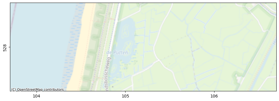
Plot the model area.

fig, ax = nlmod.plot.get_map(extent_hbossche, background="OpenStreetMap.Mapnik")

Download REGIS in our model area and create a layer model. Next convert this layer model into a model dataset using grid information using nlmod.to_model_ds.

Then we add time discretization, add the north sea to our layer model, and set default transport parameters for our transport model.

The last step is done with nlmod.gwt.prepare.set_default_transport_parameters. In this case we’re using chloride concentrations to model salinity effects, so we’ve set default parameters values for that case.

layer_model = nlmod.read.regis.get_combined_layer_models(
    extent_hbossche,
    use_regis=True,
    regis_botm_layer="MSz1",
    use_geotop=False,
    cachedir=cachedir,
    cachename="combined_layer_ds.nc",
)

# create a model ds
ds = nlmod.to_model_ds(
    layer_model,
    model_name,
    model_ws,
    delr=delr,
    delc=delc,
    transport=transport,
)

# add time discretisation
ds = nlmod.time.set_ds_time(
    ds,
    start=start_time,
    steady=False,
    steady_start=True,
    perlen=[365.0] * 10,
)

if ds.transport == 1:
    ds = nlmod.gwt.prepare.set_default_transport_parameters(
        ds, transport_type="chloride"
    )

INFO:nlmod.cache.wrapper:caching data -> combined_layer_ds.nc
INFO:nlmod.dims.base.to_model_ds:resample layer model data to structured modelgrid
INFO:nlmod.dims.layers.get_kh_kv:kv and kh both undefined in layer HLc
INFO:nlmod.dims.layers._fill_var:Filling 1080 values in active cells of kh by multipying kv with an anisotropy of 10
INFO:nlmod.dims.layers._fill_var:Filling 4785 values in active cells of kv by dividing kh by an anisotropy of 10
INFO:nlmod.dims.layers._fill_var:Filling 300 values in active cells of kh with a value of 1.0 m/day
INFO:nlmod.dims.layers._fill_var:Filling 300 values in active cells of kv with a value of 0.1 m/day

# We download the digital terrain model (AHN4)
ahn = nlmod.read.ahn.download_ahn4(ds.extent)
# calculate the average surface level in each cell
ds["ahn"] = nlmod.resample.structured_da_to_ds(ahn, ds, method="average")

Downloading tiles of AHN4:   0%|          | 0/2 [00:00<?, ?it/s]
Downloading tiles of AHN4: 100%|██████████| 2/2 [00:05<00:00,  2.87s/it]

# We download the surface level below the sea by downloading the vaklodingen
vaklodingen = nlmod.read.jarkus.get_dataset_jarkus(
    extent_hbossche,
    kind="vaklodingen",
    time="2020",
    cachedir=cachedir,
    cachename="vaklodingen.nc",
)
# calculate the average surface level in each cell
ds["vaklodingen"] = nlmod.resample.structured_da_to_ds(
    vaklodingen["z"], ds, method="average"
)

INFO:nlmod.cache.wrapper:caching data -> vaklodingen.nc
INFO:nlmod.dims.resample.structured_da_to_ds:No crs in da. Setting crs equal to ds: EPSG:28992

# calculate a new top from ahn and vaklodingen
new_top = ds["ahn"].where(~ds["ahn"].isnull(), ds["vaklodingen"])
ds = nlmod.layers.set_model_top(ds, new_top)

# we then determine the part of each cell that is covered by sea from the original ahn
ds["sea"] = nlmod.read.rws.calculate_sea_coverage(ahn, ds=ds, method="average")

Next we load chloride concentrations for our model. These are obtained from the NHI salinity dataset, where chloride concentrations for the Netherlands were determined based on observations and modeling. The full dataset 3dchlorde.nc can be downloaded from here: https://zenodo.org/record/7419219. Here we load a small dataset that was extracted from the full dataset.

This dataset does not match our model grid, so we use nearest interpolation get the chloride concentration for each of our model cells.

# cl = xr.open_dataset("../../../pwn_diep/data/3dchloride_result.nc")
cl = xr.open_dataset("./data/chloride_hbossche.nc")


# interpolate to modelgrid using nearest
cli = cl.sel(percentile="p50").interp(x=ds.x, y=ds.y, method="nearest")
cli

<xarray.Dataset> Size: 112kB
Dimensions:      (layer: 46, y: 10, x: 30)
Coordinates:
  * layer        (layer) int32 184B 1 2 3 4 5 6 7 8 ... 39 40 41 42 43 44 45 46
    z            (layer) float64 368B ...
    dz           (layer) float64 368B ...
    top          (layer) float64 368B ...
    bottom       (layer) float64 368B ...
  * y            (y) float64 80B 5.284e+05 5.284e+05 ... 5.276e+05 5.276e+05
  * x            (x) float64 240B 1.038e+05 1.038e+05 ... 1.066e+05 1.066e+05
    percentile   <U3 12B 'p50'
    dy           float64 8B ...
    dx           float64 8B ...
    spatial_ref  int64 8B 0
Data variables:
    3d-chloride  (layer, y, x) float64 110kB nan nan nan ... 1.529e+04 1.529e+04

xarray.Dataset

• Dimensions:
  • layer: 46
  • y: 10
  • x: 30
• Coordinates: (11)
  • layer
    (layer)
    int32
    1 2 3 4 5 6 7 ... 41 42 43 44 45 46

    array([ 1,  2,  3,  4,  5,  6,  7,  8,  9, 10, 11, 12, 13, 14, 15, 16, 17, 18,
           19, 20, 21, 22, 23, 24, 25, 26, 27, 28, 29, 30, 31, 32, 33, 34, 35, 36,
           37, 38, 39, 40, 41, 42, 43, 44, 45, 46], dtype=int32)

  • z
    (layer)
    float64
    ...

    [46 values with dtype=float64]

  • dz
    (layer)
    float64
    ...

    [46 values with dtype=float64]

  • top
    (layer)
    float64
    ...

    [46 values with dtype=float64]

  • bottom
    (layer)
    float64
    ...

    [46 values with dtype=float64]

  • y
    (y)
    float64
    5.284e+05 5.284e+05 ... 5.276e+05

    array([528450., 528350., 528250., 528150., 528050., 527950., 527850., 527750.,
           527650., 527550.])

  • x
    (x)
    float64
    1.038e+05 1.038e+05 ... 1.066e+05

    array([103750., 103850., 103950., 104050., 104150., 104250., 104350., 104450.,
           104550., 104650., 104750., 104850., 104950., 105050., 105150., 105250.,
           105350., 105450., 105550., 105650., 105750., 105850., 105950., 106050.,
           106150., 106250., 106350., 106450., 106550., 106650.])

  • percentile
    ()
    <U3
    'p50'

    array('p50', dtype='<U3')

  • dy
    ()
    float64
    ...

    [1 values with dtype=float64]

  • dx
    ()
    float64
    ...

    [1 values with dtype=float64]

  • spatial_ref
    ()
    int64
    0

    crs_wkt :

    PROJCS["Amersfoort / RD New",GEOGCS["Amersfoort",DATUM["Amersfoort",SPHEROID["Bessel 1841",6377397.155,299.1528128,AUTHORITY["EPSG","7004"]],AUTHORITY["EPSG","6289"]],PRIMEM["Greenwich",0,AUTHORITY["EPSG","8901"]],UNIT["degree",0.0174532925199433,AUTHORITY["EPSG","9122"]],AUTHORITY["EPSG","4289"]],PROJECTION["Oblique_Stereographic"],PARAMETER["latitude_of_origin",52.1561605555556],PARAMETER["central_meridian",5.38763888888889],PARAMETER["scale_factor",0.9999079],PARAMETER["false_easting",155000],PARAMETER["false_northing",463000],UNIT["metre",1,AUTHORITY["EPSG","9001"]],AXIS["Easting",EAST],AXIS["Northing",NORTH],AUTHORITY["EPSG","28992"]]

    spatial_ref :

    PROJCS["Amersfoort / RD New",GEOGCS["Amersfoort",DATUM["Amersfoort",SPHEROID["Bessel 1841",6377397.155,299.1528128,AUTHORITY["EPSG","7004"]],AUTHORITY["EPSG","6289"]],PRIMEM["Greenwich",0,AUTHORITY["EPSG","8901"]],UNIT["degree",0.0174532925199433,AUTHORITY["EPSG","9122"]],AUTHORITY["EPSG","4289"]],PROJECTION["Oblique_Stereographic"],PARAMETER["latitude_of_origin",52.1561605555556],PARAMETER["central_meridian",5.38763888888889],PARAMETER["scale_factor",0.9999079],PARAMETER["false_easting",155000],PARAMETER["false_northing",463000],UNIT["metre",1,AUTHORITY["EPSG","9001"]],AXIS["Easting",EAST],AXIS["Northing",NORTH],AUTHORITY["EPSG","28992"]]

    array(0)

• Data variables: (1)
  • 3d-chloride
    (layer, y, x)
    float64
    nan nan nan ... 1.529e+04 1.529e+04

    array([[[           nan,            nan,            nan, ...,
                        nan,            nan,            nan],
            [           nan,            nan,            nan, ...,
                        nan,            nan,            nan],
            [           nan,            nan,            nan, ...,
                        nan,            nan,            nan],
            ...,
            [           nan,            nan,            nan, ...,
                        nan,            nan,            nan],
            [           nan,            nan,            nan, ...,
                        nan,            nan,            nan],
            [           nan,            nan,            nan, ...,
                        nan,            nan,            nan]],
    
           [[           nan,            nan,            nan, ...,
                        nan,            nan,            nan],
            [           nan,            nan,            nan, ...,
                        nan,            nan,            nan],
            [           nan,            nan,            nan, ...,
                        nan,            nan,            nan],
    ...
             16200.41777248, 16160.00009798, 16160.00009798],
            [16389.01829574, 16379.02410467, 16379.02410467, ...,
             16200.41777248, 16160.00009798, 16160.00009798],
            [16389.01829574, 16379.02410467, 16379.02410467, ...,
             16200.41777248, 16160.00009798, 16160.00009798]],
    
           [[16134.75010521, 16134.75010521, 16134.75010521, ...,
             15442.86128429, 15442.86128429, 15442.86128429],
            [16134.75010521, 16134.75010521, 16134.75010521, ...,
             15442.86128429, 15442.86128429, 15442.86128429],
            [16134.75010521, 16134.75010521, 16134.75010521, ...,
             15442.86128429, 15442.86128429, 15442.86128429],
            ...,
            [16134.75010521, 16115.16121507, 16115.16121507, ...,
             15442.86128429, 15291.76179029, 15291.76179029],
            [16134.75010521, 16115.16121507, 16115.16121507, ...,
             15442.86128429, 15291.76179029, 15291.76179029],
            [16134.75010521, 16115.16121507, 16115.16121507, ...,
             15442.86128429, 15291.76179029, 15291.76179029]]],
          shape=(46, 10, 30))

The chloride concentration dataset also does not have the same vertical discretization as our model. In order to calculate the mean concentration in each cell in every layer of our model we use nlmod.layers.aggregate_by_weighted_mean_to_ds to calculate the weighted mean of the chloride concentration observations in each layer. We also fill the NaNs in the resulting dataset using nearest interpolation.

Finally, we add this chloride data array to our model dataset, which now has a chloride concentration for each cell in our model.

# aggregate chloride to our layer model using weighted mean
cli_da = nlmod.layers.aggregate_by_weighted_mean_to_ds(ds, cli, "3d-chloride")

# interpolate NaNs nearest
for ilay in range(cli_da.shape[0]):
    cli_da.values[ilay] = nlmod.resample.fillnan_da(
        da=cli_da.isel(layer=ilay), method="nearest"
    )

# set chloride data in model dataset, keep only layer, y and x coordinates
ds["chloride"] = ("layer", "y", "x"), cli_da.values

Now we can start building our groundwater model. We start with the Simulation object, time discretization and IMS solver.

# create simulation
sim = nlmod.sim.sim(ds)

# create time discretisation
tdis = nlmod.sim.tdis(ds, sim)

# create ims
ims = nlmod.sim.ims(sim, complexity="MODERATE")

INFO:nlmod.sim.sim.sim:creating mf6 SIM
INFO:nlmod.sim.sim.tdis:creating mf6 TDIS
INFO:nlmod.sim.sim.ims:creating mf6 IMS

Next we add the groundwater flow model.

# create groundwater flow model
gwf = nlmod.gwf.gwf(ds, sim)

# Create discretization
dis = nlmod.gwf.dis(ds, gwf)

# create node property flow
npf = nlmod.gwf.npf(ds, gwf)

# create storage
sto = nlmod.gwf.sto(ds, gwf)

# Create the initial conditions package
ic = nlmod.gwf.ic(ds, gwf, starting_head=starting_head)

# Create the output control package
oc = nlmod.gwf.oc(ds, gwf)

INFO:nlmod.gwf.gwf.gwf:creating mf6 GWF
INFO:nlmod.gwf.gwf._dis:creating mf6 DIS
INFO:nlmod.gwf.gwf.npf:creating mf6 NPF
INFO:nlmod.gwf.gwf.sto:creating mf6 STO
INFO:nlmod.gwf.gwf.ic:creating mf6 IC
INFO:nlmod.gwf.gwf.ic:adding 'starting_head' data array to ds
INFO:nlmod.gwf.gwf.oc:creating mf6 OC

We add general head boundaries to model the North Sea. We want to provide the North Sea with a chloride concentration of 18,000 mgCl-/L. This can be done by passing this value to the auxiliary keyword argument.

Note that it is also possible to reference one (or more) data arrays from the model dataset as the auxiliary variable.

If an auxiliary variable is provided and the transport attribute of the model dataset is 1 (True), nlmod automatically registers the GHB package in the ssm_sources attribute, which indicates that we need to add this package as a source (or sink) for our transport model.

# build ghb package
ghb = nlmod.gwf.ghb(
    ds,
    gwf,
    bhead=0.0,
    cond=ds["sea"] * ds["area"] / 1.0,
    auxiliary=18_000.0,
)

INFO:nlmod.gwf.gwf.ghb:creating mf6 GHB
INFO:nlmod.gwf.gwf.ghb:-> adding GHB to SSM sources list

# note that building the GHB added the package to the ssm_sources attribute
ds.ssm_sources

['ghb']

Add surface level drains to the model based on the digital elevetion model AHN.

# build surface level drain package
elev = ds["ahn"].where(ds["sea"] == 0)
drn = nlmod.gwf.surface_drain_from_ds(ds, gwf, elev=elev, resistance=10.0)

INFO:nlmod.util._get_value_from_ds_datavar:Using user-provided 'elev' and not stored data variable 'ds.ahn'

Add recharge based on timeseries measured at meteorolgical stations by KNMI.

# download knmi recharge data
knmi_ds = nlmod.read.knmi.get_recharge(ds, cachedir=ds.cachedir, cachename="recharge")
# update model dataset
ds.update(knmi_ds)

# create recharge package
rch = nlmod.gwf.rch(ds, gwf, mask=ds["sea"] == 0)

INFO:hydropandas.io.knmi.get_knmi_obs:get data from station 16 and variable RD from 2010-01-01 to 2019-12-30
INFO:hydropandas.io.knmi.get_knmi_obs:get data from station 235 and variable EV24 from 2010-01-01 to 2019-12-30
WARNING:nlmod.read.knmi.discretize_knmi:The default of hourly_precision=False will be changed to True in a future version of nlmod. Pass hourly_precision=False to retain current behavior or hourly_precision=True to adopt the future default and silence this warning.
INFO:nlmod.cache.wrapper:caching data -> recharge.nc
INFO:nlmod.gwf.gwf.rch:creating mf6 RCH

Next, the transport model is created. Note the following steps:

• The buoyancy (BUY) package is added to the groundwater flow model to take into account density effects.

• The transport model requires its own IMS solver, which also needs to be registered in the simulation.

• The advection (ADV), dispersion (DSP), mass-storage transfer (MST) and source-sink mixing (SSM) packages each obtain information from the model dataset. These variables were defined by nlmod.gwt.prepare.set_default_transport_parameters. They can be also be modified or added to the dataset by the user. Another option is to directly pass the variables to the package constructors, in which case the stored values are ignored.

if ds.transport:
    # BUY: buoyancy package for GWF model
    buy = nlmod.gwf.buy(ds, gwf)

    # GWT: groundwater transport model
    gwt = nlmod.gwt.gwt(ds, sim)

    # add IMS for GWT model and register it
    ims = nlmod.sim.ims(sim, pname="ims_gwt", filename=f"{gwt.name}.ims")
    nlmod.sim.register_ims_package(sim, gwt, ims)

    # DIS: discretization package
    dis_gwt = nlmod.gwt.dis(ds, gwt)

    # IC: initial conditions package
    ic_gwt = nlmod.gwt.ic(ds, gwt, "chloride")

    # ADV: advection package
    adv = nlmod.gwt.adv(ds, gwt)

    # DSP: dispersion package
    dsp = nlmod.gwt.dsp(ds, gwt)

    # MST: mass transfer package
    mst = nlmod.gwt.mst(ds, gwt)

    # SSM: source-sink mixing package
    ssm = nlmod.gwt.ssm(ds, gwt)

    # OC: output control
    oc_gwt = nlmod.gwt.oc(ds, gwt)

    # GWF-GWT Exchange
    gwfgwt = nlmod.gwt.gwfgwt(ds, sim)

INFO:nlmod.gwf.gwf.buy:creating mf6 BUY
INFO:nlmod.gwt.gwt.gwt:creating mf6 GWT
INFO:nlmod.sim.sim.ims:creating mf6 IMS
INFO:nlmod.gwf.gwf._dis:creating mf6 DIS
INFO:nlmod.gwt.gwt.ic:creating mf6 IC
INFO:nlmod.gwt.gwt.adv:creating mf6 ADV
INFO:nlmod.gwt.gwt.dsp:creating mf6 DSP
INFO:nlmod.gwt.gwt.mst:creating mf6 MST
INFO:nlmod.gwt.gwt.ssm:creating mf6 SSM
INFO:nlmod.gwt.gwt.oc:creating mf6 OC
INFO:nlmod.gwt.gwt.gwfgwt:creating mf6 exchange GWFGWT

Now write the model files and run the simulation.

nlmod.sim.write_and_run(sim, ds)

INFO:nlmod.sim.sim.write_and_run:write model dataset to cache
INFO:nlmod.sim.sim.write_and_run:write modflow files to model workspace
writing simulation...
  writing simulation name file...
  writing simulation tdis package...
  writing solution package ims...
  writing solution package ims_gwt...
  writing package hondsbossche.gwfgwt...
  writing model hondsbossche...
    writing model name file...
    writing package dis...
    writing package npf...
    writing package sto...
    writing package ic...
    writing package oc...
    writing package ghb...
    writing package drn...
    writing package rch...
    writing package ts_0...
    writing package buy...
  writing model hondsbossche_gwt...
    writing model name file...
    writing package dis...
    writing package ic...
    writing package adv...
    writing package dsp...
    writing package mst...
    writing package ssm...
    writing package oc...
INFO:nlmod.sim.sim.write_and_run:run model
FloPy is using the following executable to run the model: ../../../../../envs/latest/lib/python3.11/site-packages/nlmod/bin/mf6
                                   MODFLOW 6
                U.S. GEOLOGICAL SURVEY MODULAR HYDROLOGIC MODEL
                            VERSION 6.6.3 09/29/2025

   MODFLOW 6 compiled Oct 07 2025 22:51:46 with Intel(R) Fortran Intel(R) 64
   Compiler Classic for applications running on Intel(R) 64, Version 2021.7.0
                             Build 20220726_000000

This software has been approved for release by the U.S. Geological 
Survey (USGS). Although the software has been subjected to rigorous 
review, the USGS reserves the right to update the software as needed 
pursuant to further analysis and review. No warranty, expressed or 
implied, is made by the USGS or the U.S. Government as to the 
functionality of the software and related material nor shall the 
fact of release constitute any such warranty. Furthermore, the 
software is released on condition that neither the USGS nor the U.S. 
Government shall be held liable for any damages resulting from its 
authorized or unauthorized use. Also refer to the USGS Water 
Resources Software User Rights Notice for complete use, copyright, 
and distribution information.

 
 MODFLOW runs in SEQUENTIAL mode
 
 Run start date and time (yyyy/mm/dd hh:mm:ss): 2026/05/13 15:14:22
 
 Writing simulation list file: mfsim.lst
 Using Simulation name file: mfsim.nam
    Solving:  Stress period:     1    Time step:     1
    Solving:  Stress period:     2    Time step:     1
    Solving:  Stress period:     3    Time step:     1
    Solving:  Stress period:     4    Time step:     1
    Solving:  Stress period:     5    Time step:     1
    Solving:  Stress period:     6    Time step:     1
    Solving:  Stress period:     7    Time step:     1
    Solving:  Stress period:     8    Time step:     1
    Solving:  Stress period:     9    Time step:     1
    Solving:  Stress period:    10    Time step:     1
 
 Run end date and time (yyyy/mm/dd hh:mm:ss): 2026/05/13 15:14:23
 Elapsed run time:  0.771 Seconds
 
 Normal termination of simulation.

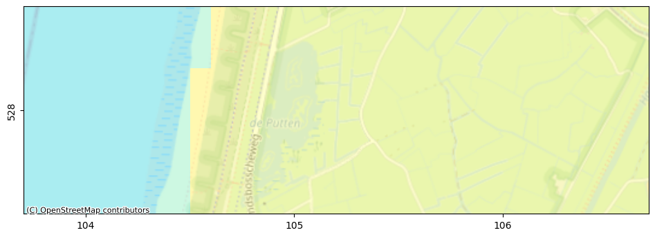
Visualize the model input, specifically the boundary conditions.

# plot using flopy
fig, ax = nlmod.plot.get_map(extent_hbossche, background="OpenStreetMap.Mapnik")
pmv = fp.plot.PlotMapView(model=gwf, layer=0, ax=ax)
# pc = pmv.plot_array(c.isel(time=0), cmap="Spectral_r")
pmv.plot_bc("GHB", plotAll=True, alpha=0.1, label="GHB")
pmv.plot_bc("DRN", plotAll=True, alpha=0.1, label="DRN")
# pmv.plot_bc("RCH", plotAll=True, alpha=0.1, label="RCH")
municipalities.plot(edgecolor="k", facecolor="none", ax=ax)
pmv.plot_grid(linewidth=0.25)
ax.set_xlabel("x [km RD]")
ax.set_ylabel("y [km RD]");

---------------------------------------------------------------------------
NameError                                 Traceback (most recent call last)
Cell In[20], line 8
      4 # pc = pmv.plot_array(c.isel(time=0), cmap="Spectral_r")
      5 pmv.plot_bc("GHB", plotAll=True, alpha=0.1, label="GHB")
      6 pmv.plot_bc("DRN", plotAll=True, alpha=0.1, label="DRN")
      7 # pmv.plot_bc("RCH", plotAll=True, alpha=0.1, label="RCH")
----> 8 municipalities.plot(edgecolor="k", facecolor="none", ax=ax)
      9 pmv.plot_grid(linewidth=0.25)
     10 ax.set_xlabel("x [km RD]")
     11 ax.set_ylabel("y [km RD]");

NameError: name 'municipalities' is not defined

Load the calculated heads and concentrations.

h = nlmod.gwf.output.get_heads_da(ds)
c = nlmod.gwt.output.get_concentration_da(ds)

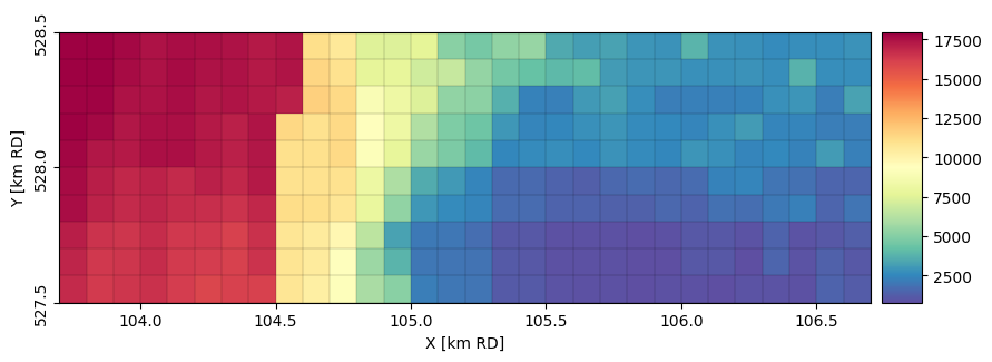
# calculate concentration at groundwater surface
ctop = nlmod.gwt.get_concentration_at_gw_surface(c)

Plot the concentration at groundwater surface level.

ax = nlmod.plot.map_array(
    ctop.isel(time=-1),
    ds,
    ilay=0,
    cmap="Spectral_r",
)
municipalities.plot(edgecolor="k", facecolor="none", ax=ax)

---------------------------------------------------------------------------
NameError                                 Traceback (most recent call last)
Cell In[22], line 7
      3     ds,
      4     ilay=0,
      5     cmap="Spectral_r",
      6 )
----> 7 municipalities.plot(edgecolor="k", facecolor="none", ax=ax)

NameError: name 'municipalities' is not defined

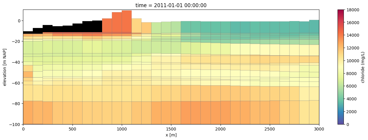
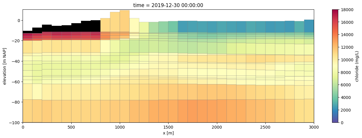
Plot a cross-section along (x) showing the calculated concentration in the model.

y = (ds.extent[2] + ds.extent[3]) / 2 + 0.1
line = [(ds.extent[0], y), (ds.extent[1], y)]
zmin = -150.0
zmax = 10.0

for time_idx in [0, -1]:
    # plot using flopy
    fig, ax = plt.subplots(1, 1, figsize=(16, 5))
    pmv = fp.plot.PlotCrossSection(model=gwf, line={"line": line})
    pc = pmv.plot_array(
        c.isel(time=time_idx), cmap="Spectral_r", vmin=0.0, vmax=18_000.0
    )
    pmv.plot_bc("GHB", color="k", zorder=10)
    pmv.plot_grid(linewidth=0.25)
    cbar = fig.colorbar(pc, ax=ax)
    cbar.set_label("chloride (mg/L)")
    ax.set_ylim(bottom=-100)
    ax.set_xlabel("x [m]")
    ax.set_ylabel("elevation [m NAP]")
    # convert to pandas timestamp for prettier printing
    ax.set_title(f"time = {pd.Timestamp(c.time.isel(time=time_idx).values)}")

Converting calculated heads (which represent point water heads) to equivalent freshwater heads, and vice versa, can be done with the following functions in nlmod.

hf = nlmod.gwt.output.freshwater_head(ds, h, c)
hp = nlmod.gwt.output.pointwater_head(ds, hf, c)

xr.testing.assert_allclose(h, hp)