The Lake Package
The Lake (LAK) package can be used to model large surface water bodies with a single, uniform stage. The lake water balance is computed, and the resulting lake stage is determined by all inflows to and outflows from the lake. Several management options are available. Users can specify inflows and outflows, redirect discharge from other packages (e.g. DRN) to the lake, impose a fixed stage, or add a weir to control maximum water levels.
In this example, the Henschotermeer lake in the Utrechtse Heuvelrug is modelled using the Lake package. For demonstration purposes, a weir is included with an invert level of 7.0 m MSL.
import os
import pandas as pd
import xarray as xr
import matplotlib.pyplot as plt
import matplotlib
import flopy
import nlmod
# set up pretty logging and show package versions
nlmod.util.get_color_logger()
nlmod.show_versions()
Python version     : 3.11.14
NumPy version      : 2.4.4
Xarray version     : 2026.4.0
Matplotlib version : 3.10.9
Flopy version      : 3.10.0

nlmod version      : 0.11.3dev
Define model extent and model workspace
extent = [152_000, 156_000, 453_500, 456_000]
model_name = "henschotermeer"
model_ws = "01_lake"
figdir, cachedir = nlmod.util.get_model_dirs(model_ws)
Download and prepare data
We download:
the layers from the subsurface model Regis
the surface level data from AHN5
the layer ‘waterdeel’ from the Basisregistratie Grootschalige Toppgrafie (BGT)
level areas from waterboard Vallei en Veluwe
regis = nlmod.read.download_regis(extent, cachedir=cachedir, cachename="regis")
ahn = nlmod.read.ahn.download_ahn5(extent, cachedir=cachedir, cachename="ahn5")
bgt = nlmod.read.bgt.download_bgt(extent, cachedir=cachedir, cachename="bgt")
bgt = bgt.set_index("identificatie")
la = nlmod.read.waterboard.download_data(
    "Vallei en Veluwe",
    "level_areas",
    extent=extent,
    cachedir=cachedir,
    cachename="la_v_en_v",
)
WARNING:nlmod.dims.layers.remove_layer_dim_from_top:Botm of layer is not equal to top of deeper layer in 1 cells
INFO:nlmod.cache.wrapper:caching data -> regis.nc
WARNING:rasterio._env.open:CPLE_AppDefined in HTTP response code on https://fsn1.your-objectstorage.com/hwh-ahn/AHN5/02b_DTM_5m/2023_M5_32DZ1.xml: 403
WARNING:rasterio._env.open:CPLE_AppDefined in HTTP response code on https://fsn1.your-objectstorage.com/hwh-ahn/AHN5/02b_DTM_5m/2023_M5_32DZ1.XML: 403
WARNING:rasterio._env.open:CPLE_AppDefined in HTTP response code on https://fsn1.your-objectstorage.com/hwh-ahn/AHN5/02b_DTM_5m/2023_M5_32DZ1.TIF.aux.xml: 403
WARNING:rasterio._env.open:CPLE_AppDefined in HTTP response code on https://fsn1.your-objectstorage.com/hwh-ahn/AHN5/02b_DTM_5m/2023_M5_32DZ1.aux: 403
WARNING:rasterio._env.open:CPLE_AppDefined in HTTP response code on https://fsn1.your-objectstorage.com/hwh-ahn/AHN5/02b_DTM_5m/2023_M5_32DZ1.AUX: 403
WARNING:rasterio._env.open:CPLE_AppDefined in HTTP response code on https://fsn1.your-objectstorage.com/hwh-ahn/AHN5/02b_DTM_5m/2023_M5_32DZ1.TIF.aux: 403
WARNING:rasterio._env.open:CPLE_AppDefined in HTTP response code on https://fsn1.your-objectstorage.com/hwh-ahn/AHN5/02b_DTM_5m/2023_M5_32DZ1.TIF.AUX: 403
WARNING:rasterio._env.open:CPLE_AppDefined in HTTP response code on https://fsn1.your-objectstorage.com/hwh-ahn/AHN5/02b_DTM_5m/2023_M5_32DZ2.xml: 403
WARNING:rasterio._env.open:CPLE_AppDefined in HTTP response code on https://fsn1.your-objectstorage.com/hwh-ahn/AHN5/02b_DTM_5m/2023_M5_32DZ2.XML: 403
WARNING:rasterio._env.open:CPLE_AppDefined in HTTP response code on https://fsn1.your-objectstorage.com/hwh-ahn/AHN5/02b_DTM_5m/2023_M5_32DZ2.TIF.aux.xml: 403
WARNING:rasterio._env.open:CPLE_AppDefined in HTTP response code on https://fsn1.your-objectstorage.com/hwh-ahn/AHN5/02b_DTM_5m/2023_M5_32DZ2.aux: 403
WARNING:rasterio._env.open:CPLE_AppDefined in HTTP response code on https://fsn1.your-objectstorage.com/hwh-ahn/AHN5/02b_DTM_5m/2023_M5_32DZ2.AUX: 403
WARNING:rasterio._env.open:CPLE_AppDefined in HTTP response code on https://fsn1.your-objectstorage.com/hwh-ahn/AHN5/02b_DTM_5m/2023_M5_32DZ2.TIF.aux: 403
WARNING:rasterio._env.open:CPLE_AppDefined in HTTP response code on https://fsn1.your-objectstorage.com/hwh-ahn/AHN5/02b_DTM_5m/2023_M5_32DZ2.TIF.AUX: 403
INFO:nlmod.cache.wrapper:caching data -> ahn5.nc
INFO:nlmod.cache.decorator:caching data -> bgt.pklz
INFO:nlmod.cache.decorator:caching data -> la_v_en_v.pklz
Downloading tiles of AHN5:   0%|          | 0/2 [00:00<?, ?it/s]
Downloading tiles of AHN5: 100%|██████████| 2/2 [00:02<00:00,  1.32s/it]
Warning 1: HTTP response code on https://fsn1.your-objectstorage.com/hwh-ahn/AHN5/02b_DTM_5m/2023_M5_32DZ1.TIF.msk: 403
Warning 1: HTTP response code on https://fsn1.your-objectstorage.com/hwh-ahn/AHN5/02b_DTM_5m/2023_M5_32DZ1.TIF.MSK: 403
Warning 1: HTTP response code on https://fsn1.your-objectstorage.com/hwh-ahn/AHN5/02b_DTM_5m/2023_M5_32DZ2.TIF.msk: 403
Warning 1: HTTP response code on https://fsn1.your-objectstorage.com/hwh-ahn/AHN5/02b_DTM_5m/2023_M5_32DZ2.TIF.MSK: 403
Combine surface water data
We add information from AHN and level areas to BGT-data.
columns = ["summer_stage", "winter_stage"]
bgt = nlmod.util.gdf_intersection_join(
    la,
    bgt,
    columns=columns,
    min_total_overlap=0.0,
    desc=f"Adding {columns} to bgt-data",
)

bgt = nlmod.gwf.surface_water.add_min_ahn_to_gdf(bgt, ahn, buffer=5.0)
bgt["summer_stage"] = bgt[["summer_stage", "ahn_min"]].max(1)
bgt["winter_stage"] = bgt[["winter_stage", "ahn_min"]].max(1)
bgt["stage"] = bgt[["summer_stage", "winter_stage"]].mean(1)

bgt["lake"] = None
henschotermeer = bgt.area.idxmax()  # 'W0662.ce4627405cb242ee8533946265644bb3'
bgt.loc[henschotermeer, "lake"] = "Henschotermeer"
Adding ['summer_stage', 'winter_stage'] to bgt-data:   0%|          | 0/612 [00:00<?, ?it/s]
Adding ['summer_stage', 'winter_stage'] to bgt-data: 100%|██████████| 612/612 [00:00<00:00, 995.01it/s]
Generate a model dataset
We generate a model dataset with the same resolution as REGIS (100 x 100 m) and refine the model with level 2 (to 25x25 m) around the Henschotermeer.
ds = nlmod.to_model_ds(regis, model_name=model_name, model_ws=model_ws)

# drop layers below "PZWAz3"
ds = ds.sel(layer=ds.layer.loc[:"PZWAz3"])

# refine around the edge of the lakes
bgt_lake_boundary = bgt.loc[~bgt["lake"].isna()].copy()
bgt_lake_boundary.geometry = bgt_lake_boundary.boundary
ds = nlmod.grid.refine(ds, refinement_features=[(bgt_lake_boundary, 2)])
INFO:nlmod.dims.base.to_model_ds:resample layer model data to structured modelgrid
fetched release '23.0' info from MODFLOW-ORG/executables
downloading 'https://github.com/MODFLOW-ORG/executables/releases/download/23.0/linux.zip' to '/tmp/tmpyejqntle/modflow_executables-23.0-linux.zip'
extracting 25 files to '/home/docs/checkouts/readthedocs.org/user_builds/nlmod/envs/latest/lib/python3.11/site-packages/nlmod/bin'
crt (1.3.1)         mflgr (2.0.0)       mp6 (6.0.1)         vs2dt (3.3)
gridgen (1.0.02)    mflgrdbl (2.0.0)    mp7 (7.2.001)       zbud6 (6.6.3)
libmf6.so (6.6.3)   mfnwt (1.3.0)       mt3dms (5.3.0)      zonbud3 (3.01)
mf2000 (1.19.01)    mfnwtdbl (1.3.0)    mt3dusgs (1.1.0)    zonbudusg (1.5)
mf2005 (1.12.00)    mfusg (1.5)         sutra (4.0)
mf2005dbl (1.12.00) mfusgdbl (1.5)      swtv4 (4.00.05)
mf6 (6.6.3)         mfusg_gsi (2.5.0)   triangle (1.6)
wrote new flopy metadata file: '/home/docs/.local/share/flopy/get_modflow.json'
INFO:nlmod.dims.layers.get_kh_kv:kv and kh both undefined in layer DTc
INFO:nlmod.dims.layers._fill_var:Filling 6842 values in active cells of kh by multipying kv with an anisotropy of 10
INFO:nlmod.dims.layers._fill_var:Filling 16524 values in active cells of kv by dividing kh by an anisotropy of 10
INFO:nlmod.dims.layers._fill_var:Filling 648 values in active cells of kh with a value of 1.0 m/day
INFO:nlmod.dims.layers._fill_var:Filling 648 values in active cells of kv with a value of 0.1 m/day
INFO:nlmod.dims.grid.refine:create vertex grid using gridgen
INFO:nlmod.dims.grid.ds_to_gridprops:resample model Dataset to vertex modelgrid
Split surface water shapes by grid
We split the surface water shapes by the modelgrid using the method nlmod.grid.gdf_to_grid. We then seperate the resulting features to a variable lak_grid for the LAK-package and a variable drn_grid for the DRN-pacakge.
bgt_grid = nlmod.grid.gdf_to_grid(bgt, ds).set_index("cellid")
mask = bgt_grid["lake"].isna()
drn_grid = bgt_grid[mask].copy()
lak_grid = bgt_grid[~mask].copy()
assert not lak_grid.index.duplicated().any()
# only keep cells where ahlf of the are of the cell is covered by lakes
mask = lak_grid.area > 0.5 * ds["area"].sel(icell2d=lak_grid.index)
lak_grid = lak_grid[mask]
# set the geometry to the entire cell
gi = flopy.utils.GridIntersect(nlmod.grid.modelgrid_from_ds(ds))
lak_grid.geometry = gi.geoms[lak_grid.index]

# remove drains that overlap with the lake
drn_grid = drn_grid.loc[~drn_grid.index.isin(lak_grid.index)]
Intersecting with grid:   0%|          | 0/612 [00:00<?, ?it/s]
Intersecting with grid: 100%|██████████| 612/612 [00:01<00:00, 310.67it/s]
Improve model dataset
Set the top of the model
The lake’s bottom elevation is defined by the top of the model. For this reason, we set the top of the model to 3.0 m MSL at the lake cells, which corresponds to the estimated lake bottom. The bottom elevation is particularly important in areas where the lake may dry out, which can also lead to convergence issues in the model. In this case, a bottom elevation of 3.0 m MSL is sufficiently deep, ensuring that the lake remains saturated throughout the transient simulation.
top = nlmod.resample.structured_da_to_ds(nlmod.resample.fillnan_da(ahn), ds)
# The botom of the lake is at 3.0 m NAP
top[lak_grid.index] = 3.0
ds = nlmod.layers.set_model_top(ds, top)
Set time dimension
Before downloading meteorological data, we define the time dimension of our model dataset. The simulation covers five years, from the beginning of 2020 to the beginning of 2025, using monthly stress periods. The model is initialized with a steady-state stress period representing the mean meteorological conditions of 2019.
time = pd.date_range("2020", "2025", freq="MS")
ds = nlmod.time.set_ds_time(ds, start="2019", time=time)
Download recharge data
We use the method nlmod.read.knmi.get_recharge to download meteorological data. Instead of calculating recharge as precipitation minus evaporation, we retrieve both variables separately by setting method="separate". Since our model area is relatively small, we represent it using a single meteorological and precipitation station (most_common_station=True). The variables recharge and evaporation are defined per station rather than for each model cell, which is achieved with add_stn_dimensions=True. Finally, to adopt the new default and suppress warnings about hourly precision, we set hourly_precision=True.
rch_ds = nlmod.read.knmi.get_recharge(
    ds=ds,
    method="separate",
    most_common_station=True,
    add_stn_dimensions=True,
    hourly_precision=True,
    cachedir=cachedir,
    cachename="knmi",
)
ds.update(rch_ds)

ds["starting_head"] = xr.full_like(ds.botm, 5.0)
INFO:hydropandas.io.knmi.get_knmi_obs:get data from station 546 and variable RD from 2019-01-01 to 2025-01-01
INFO:hydropandas.io.knmi.get_knmi_obs:get data from station 265 and variable EV24 from 2019-01-01 to 2025-01-01
INFO:hydropandas.io.knmi.fill_missing_measurements:station 265 has no measurements between 2019-01-01 00:00:00 and 2025-01-01 00:00:00 trying to get measurements from nearest station -> 260
INFO:nlmod.cache.wrapper:caching data -> knmi.nc
Generate and run model
Generate a FloPy sim and gwf
sim = nlmod.sim.sim(ds)  # simulation
tdis = nlmod.sim.tdis(ds, sim)  # time discretization
ims = nlmod.sim.ims(
    sim,
    complexity="COMPLEX",
    inner_dvclose=0.01, # needed so lake balance is correct
    outer_dvclose=0.01, # needed so lake balance is correct
    #rcloserecord=[0.01, "STRICT"],
)  # ims solver
gwf = nlmod.gwf.gwf(ds, sim, under_relaxation=True)  # groundwater flow model
dis = nlmod.gwf.dis(ds, gwf)  # spatial discretization
npf = nlmod.gwf.npf(ds, gwf)  # node property flow
sto = nlmod.gwf.sto(ds, gwf)  # storage
ic = nlmod.gwf.ic(ds, gwf)  # initial conditions
oc = nlmod.gwf.oc(ds, gwf)  # output control
INFO:nlmod.sim.sim.sim:creating mf6 SIM
INFO:nlmod.sim.sim.tdis:creating mf6 TDIS
INFO:nlmod.sim.sim.ims:creating mf6 IMS
INFO:nlmod.gwf.gwf.gwf:creating mf6 GWF
INFO:nlmod.gwf.gwf._disv:creating mf6 DISV
INFO:nlmod.gwf.gwf.npf:creating mf6 NPF
INFO:nlmod.gwf.gwf.sto:creating mf6 STO
INFO:nlmod.gwf.gwf.ic:creating mf6 IC
INFO:nlmod.gwf.gwf.oc:creating mf6 OC
Meteorological stresses
rch = nlmod.gwf.rch(ds, gwf)
evt = nlmod.gwf.evt(ds, gwf)
INFO:nlmod.gwf.gwf.rch:creating mf6 RCH
INFO:nlmod.gwf.gwf.evt:creating mf6 EVT
INFO:nlmod.gwf.recharge.ds_to_evt:Setting evaporation surface to 1 meter below top
INFO:nlmod.gwf.recharge.ds_to_evt:Setting extinction depth to 1 meter below surface
Lake package for the Henschotermeer
# %%
lak_resistance = 10.0  # days
lak_grid["clake"] = lak_resistance
lak_grid["strt"] = 6.0
lak_grid["lakeout"] = -1
lak_grid["outlet_invert"] = 7.0
nlmod.gwf.lake_from_gdf(
    gwf,
    lak_grid,
    ds,
    rainfall=ds["recharge"].to_pandas().iloc[:, 0],
    evaporation=ds["evaporation"].to_pandas().iloc[:, 0] * 1.25,
    boundname_column="lake",
    #maximum_stage_change=0.000001,
    #maximum_iterations=200,
);
Drain package for all other surface water
drn_resistance = 1.0  # days
drn_grid["cond"] = drn_grid.area / drn_resistance
spd = nlmod.gwf.surface_water.build_spd(drn_grid, "DRN", ds)
drn = flopy.mf6.ModflowGwfdrn(gwf, stress_period_data={0: spd})
Building stress period data DRN:   0%|          | 0/1369 [00:00<?, ?it/s]
Building stress period data DRN: 100%|██████████| 1369/1369 [00:00<00:00, 6590.48it/s]
Write input-files and run Modflow 6
nlmod.sim.write_and_run(sim, ds)
INFO:nlmod.sim.sim.write_and_run:write model dataset to cache
INFO:nlmod.sim.sim.write_and_run:write modflow files to model workspace
writing simulation...
  writing simulation name file...
  writing simulation tdis package...
  writing solution package ims...
  writing model henschotermeer...
    writing model name file...
    writing package disv...
    writing package npf...
    writing package sto...
    writing package ic...
    writing package oc...
    writing package rch...
    writing package ts_0...
    writing package evt...
    writing package ts_1...
    writing package lak...
    writing package obs_0...
    writing package drn_0...
INFORMATION: maxbound in ('', 'drn', 'dimensions') changed to 1369 based on size of stress_period_data
INFO:nlmod.sim.sim.write_and_run:run model
FloPy is using the following executable to run the model: ../../../../../envs/latest/lib/python3.11/site-packages/nlmod/bin/mf6
                                   MODFLOW 6
                U.S. GEOLOGICAL SURVEY MODULAR HYDROLOGIC MODEL
                            VERSION 6.6.3 09/29/2025

   MODFLOW 6 compiled Oct 07 2025 22:51:46 with Intel(R) Fortran Intel(R) 64
   Compiler Classic for applications running on Intel(R) 64, Version 2021.7.0
                             Build 20220726_000000

This software has been approved for release by the U.S. Geological
Survey (USGS). Although the software has been subjected to rigorous
review, the USGS reserves the right to update the software as needed
pursuant to further analysis and review. No warranty, expressed or
implied, is made by the USGS or the U.S. Government as to the
functionality of the software and related material nor shall the
fact of release constitute any such warranty. Furthermore, the
software is released on condition that neither the USGS nor the U.S.
Government shall be held liable for any damages resulting from its
authorized or unauthorized use. Also refer to the USGS Water
Resources Software User Rights Notice for complete use, copyright,
and distribution information.


 MODFLOW runs in SEQUENTIAL mode

 Run start date and time (yyyy/mm/dd hh:mm:ss): 2026/05/13 15:05:23

 Writing simulation list file: mfsim.lst
 Using Simulation name file: mfsim.nam
    Solving:  Stress period:     1    Time step:     1
    Solving:  Stress period:     2    Time step:     1
    Solving:  Stress period:     3    Time step:     1
    Solving:  Stress period:     4    Time step:     1
    Solving:  Stress period:     5    Time step:     1
    Solving:  Stress period:     6    Time step:     1
    Solving:  Stress period:     7    Time step:     1
    Solving:  Stress period:     8    Time step:     1
    Solving:  Stress period:     9    Time step:     1
    Solving:  Stress period:    10    Time step:     1
    Solving:  Stress period:    11    Time step:     1
    Solving:  Stress period:    12    Time step:     1
    Solving:  Stress period:    13    Time step:     1
    Solving:  Stress period:    14    Time step:     1
    Solving:  Stress period:    15    Time step:     1
    Solving:  Stress period:    16    Time step:     1
    Solving:  Stress period:    17    Time step:     1
    Solving:  Stress period:    18    Time step:     1
    Solving:  Stress period:    19    Time step:     1
    Solving:  Stress period:    20    Time step:     1
    Solving:  Stress period:    21    Time step:     1
    Solving:  Stress period:    22    Time step:     1
    Solving:  Stress period:    23    Time step:     1
    Solving:  Stress period:    24    Time step:     1
    Solving:  Stress period:    25    Time step:     1
    Solving:  Stress period:    26    Time step:     1
    Solving:  Stress period:    27    Time step:     1
    Solving:  Stress period:    28    Time step:     1
    Solving:  Stress period:    29    Time step:     1
    Solving:  Stress period:    30    Time step:     1
    Solving:  Stress period:    31    Time step:     1
    Solving:  Stress period:    32    Time step:     1
    Solving:  Stress period:    33    Time step:     1
    Solving:  Stress period:    34    Time step:     1
    Solving:  Stress period:    35    Time step:     1
    Solving:  Stress period:    36    Time step:     1
    Solving:  Stress period:    37    Time step:     1
    Solving:  Stress period:    38    Time step:     1
    Solving:  Stress period:    39    Time step:     1
    Solving:  Stress period:    40    Time step:     1
    Solving:  Stress period:    41    Time step:     1
    Solving:  Stress period:    42    Time step:     1
    Solving:  Stress period:    43    Time step:     1
    Solving:  Stress period:    44    Time step:     1
    Solving:  Stress period:    45    Time step:     1
    Solving:  Stress period:    46    Time step:     1
    Solving:  Stress period:    47    Time step:     1
    Solving:  Stress period:    48    Time step:     1
    Solving:  Stress period:    49    Time step:     1
    Solving:  Stress period:    50    Time step:     1
    Solving:  Stress period:    51    Time step:     1
    Solving:  Stress period:    52    Time step:     1
    Solving:  Stress period:    53    Time step:     1
    Solving:  Stress period:    54    Time step:     1
    Solving:  Stress period:    55    Time step:     1
    Solving:  Stress period:    56    Time step:     1
    Solving:  Stress period:    57    Time step:     1
    Solving:  Stress period:    58    Time step:     1
    Solving:  Stress period:    59    Time step:     1
    Solving:  Stress period:    60    Time step:     1
    Solving:  Stress period:    61    Time step:     1

 Run end date and time (yyyy/mm/dd hh:mm:ss): 2026/05/13 15:05:35
 Elapsed run time: 12.408 Seconds

 Normal termination of simulation.
Post-processing
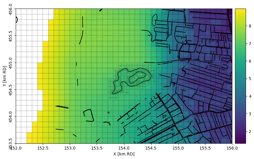
Plot the head in the top layer
We plot the time-averaged head in the first model layer, BXz2. This layer is absent in the western part of the model domain, which is why this area appears white in the figure. Surface water features (bgt) are plotted on top of the map for reference. The finer model cells along the shoreline of Lake Henschotermeer are clearly visible.
head = nlmod.gwf.get_heads_da(ds)
ax = nlmod.plot.map_array(head.sel(layer="BXz2").mean("time"), ds=ds)
bgt.plot(edgecolor='k', facecolor='none', ax=ax);
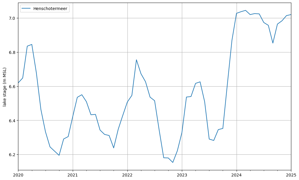
Plot the Lake stage
If the parameter boundname_column is specified in nlmod.gwf.lake_from_gdf, a CSV file named lak_STAGE.csv is generated containing observations of lake stages. Below, we plot the lake stage. Due to the wet conditions during the winter of 2023/2024, the lake level rises to 7.0 m MSL. At this elevation, the weir becomes active, preventing any further significant increase in lake stage.
lak_stage = pd.read_csv(os.path.join(ds.model_ws, "lak_STAGE.csv"), index_col=0)
lak_stage.index = pd.to_datetime(ds.time.start) + pd.to_timedelta(lak_stage.index, "d")
lak_stage.columns = [x.capitalize() for x in lak_stage.columns]

f, ax = plt.subplots(figsize=(10, 6), layout="constrained")
lak_stage.plot(ax=ax)
ax.set_xlabel("")
ax.set_ylabel("lake stage (m MSL)")
ax.grid()
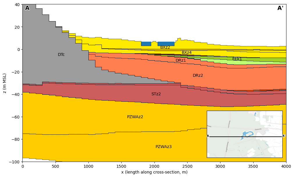
Plot a cross-section
We plot a west–east cross-section at y = 454 612, showing the model layers. We can see the Utrechtse Heuvelrug on the left (west), with decreasing surface level eastwards. The lake “Henschotermeer” is displayed in blue, using the mean lake stage over the simulation period.
f, ax = plt.subplots(figsize=(10, 6), layout="constrained")
line = [(extent[0], 454_612), (extent[1], 454_612)]
dcs = nlmod.plot.DatasetCrossSection(ds, line, ax=ax, zmin=-100)
dcs.plot_layers(colors=nlmod.read.regis.get_legend())
dcs.plot_grid(vertical=False, lw=0.5)
dcs.label_layers()

lak_gdf = lak_grid.dissolve("lake")


def plot_lake_in_cs(linestring, dcs, height, ax, color="C0", zorder=0):
    xy = (dcs.line.project(linestring.boundary.geoms[0]), dcs.zmin)
    width = dcs.line.project(linestring.boundary.geoms[1]) - xy[0]
    rect = matplotlib.patches.Rectangle(
        xy, width, height, color=color, zorder=zorder
    )
    ax.add_patch(rect)

# plot the lake
for lake in bgt.loc[~bgt.lake.isna(), "lake"].unique():
    mean_lake_stage = lak_stage[lake].mean()
    ylim = ax.get_ylim()
    height = mean_lake_stage - ylim[0]
    mask = bgt.lake == lake
    for geom in lak_gdf.loc[[lake]].intersection(dcs.line).geometry.values:
        if geom.geom_type == "MultiLineString":
            for geom_line in geom.geoms:
                plot_lake_in_cs(geom_line, dcs, height, ax)
        else:
            plot_lake_in_cs(geom, dcs, height, ax)


axes_bounds = nlmod.plot.get_inset_map_bounds(ax, extent, height=0.3)
mapax = nlmod.plot.inset_map(ax, extent, axes_bounds=axes_bounds)
nlmod.plot.add_xsec_line_and_labels(line, ax, mapax)
ax.set_xlabel("x (length along cross-section, m)")
ax.set_ylabel("z (m MSL)");
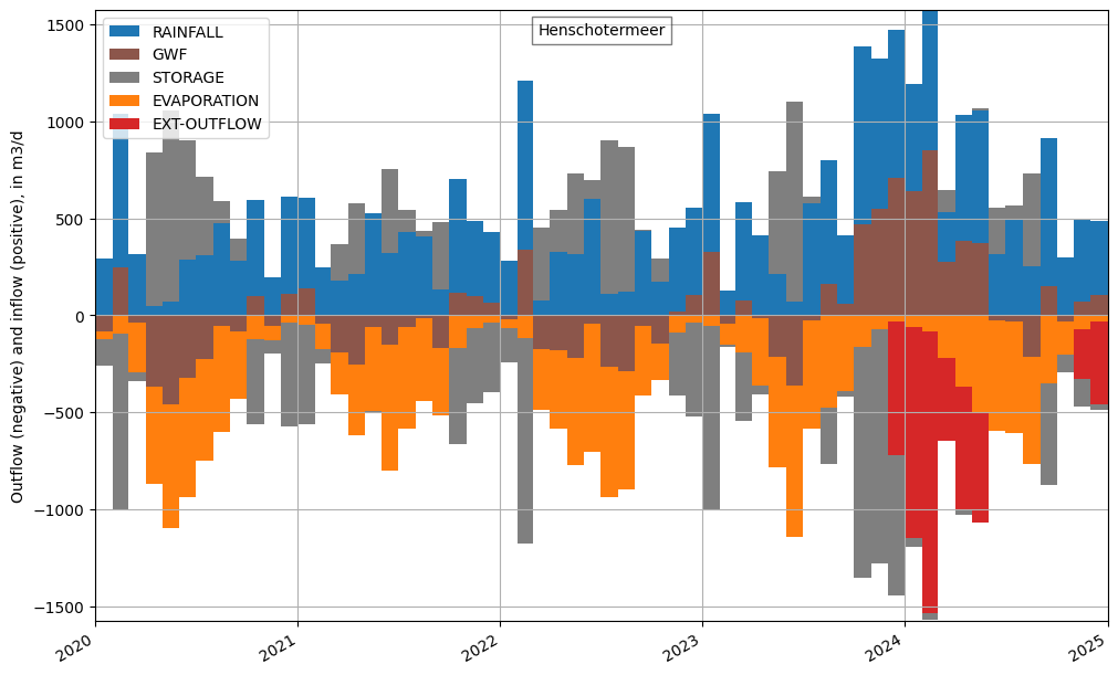
Plot a water balance of the lake
The main advantage of using the LAK package is that the lake water balance is explicitly accounted for. This water balance is saved in the file lak.bgt. Below, we read this file and plot the results. The primary fluxes into and out of the lake are rainfall (blue) and evaporation (orange), which are model inputs. The calculated flux between the lake and the groundwater (GWF, brown) shows a substantial contribution of groundwater flow to the lake during the winter of 2023/2024. This inflow, and rainfall, causes the lake stage to rise, resulting in a negative storage term (grey). From the winter of 2023/2024 onward, the weir becomes active, causing external outflow of water (red).
fname = os.path.join(ds.model_ws, "lak.bgt")
cbf_lak = nlmod.gwf.output.get_cellbudgetfile(fname=fname, ds=ds)

# read budgets
lake_bgt = {}
for rn in cbf_lak.get_unique_record_names():
    key = rn.strip().decode()
    lake_bgt[key] = cbf_lak.get_data(text=rn)

colors = {
    "GWF": "tab:brown",
    "RAINFALL": "tab:blue",
    "CONSTANT": "tab:purple",
    "EVAPORATION": "tab:orange",
    "STORAGE": "tab:gray",
    "FROM-MVR": "tab:green",
    "EXT-OUTFLOW": "tab:red",
}


for name in lak_grid["lake"].unique():
    lakeno = int(lak_grid.loc[lak_grid["lake"] == name, "lakeno"].iloc[0])
    # generate a DataFrame
    data = {}
    for key in lake_bgt.keys():
        data[key] = [x[x["node"] == lakeno + 1]["q"].sum() for x in lake_bgt[key]]

    index = pd.to_datetime(ds.time.start) + pd.to_timedelta(cbf_lak.get_times(), "d")
    df = pd.DataFrame(data, index=index)

    f, ax = plt.subplots(figsize=(10, 6), layout="constrained")

    dfs = df.copy()
    dfs.index = [pd.to_datetime(ds.time.start)] + list(df.index[:-1])
    df_block = pd.concat((df, dfs)).sort_index(kind="mergesort")

    inflow = df_block.where(df_block > 0, 0.0)
    inflow = inflow.loc[:, ~(inflow == 0).all()]

    outflow = df_block.where(df_block < 0, 0.0)
    outflow = outflow.loc[:, ~(outflow == 0).all()]

    ymax = max(inflow.sum(1).max(), outflow.sum(1).max())

    inflow.plot.area(color=colors, ax=ax, linewidth=0)
    handles_in, labels_in = ax.get_legend_handles_labels()
    ax.set_ylim(-ymax, ymax)
    outflow.plot.area(color=colors, ax=ax, linewidth=0)
    ax.set_ylim(-ymax, ymax)

    ax.set_xlim(ds.time.data[0], ds.time.data[-1])
    ax.set_ylabel("Outflow (negative) and inflow (positive), in m3/d")
    nlmod.plot.title_inside(name, ax=ax)

    # remove double legend entries
    handles_all, labels_all = ax.get_legend_handles_labels()

    handles = handles_in[::-1]
    labels = labels_in[::-1]

    # move storage to the middle of the legend
    index = labels.index("STORAGE")
    handles.append(handles.pop(index))
    labels.append(labels.pop(index))
    for handle, label in zip(handles_all, labels_all):
        if label not in labels:
            handles.append(handle)
            labels.append(label)

    ax.legend(handles, labels, loc=2)
    ax.grid()