Plot methods in nlmod
This notebook shows different methods of plotting data with nlmod.
There are many ways to plot data and it depends on the type of data and plot which of these method is the most convenient:
using
nlmod.plotutilitiesusing
flopyplot methodsusing
xarrayplot methods
The default plot methods in nlmod use a model Dataset as input (this is an xarray
Dataset with some required variables and attributes). These plotting methods are
accessible through nlmod.plot.
Flopy contains its own plotting utilities and nlmod contains some wrapper functions that
use flopy’s plotting utilities under the hood. These require a flopy modelgrid or model
object. These plotting methods are accessible through nlmod.plot.flopy.
Finally, xarray also allows plotting of data with .plot(). This is used in a few
cases in this notebook but for more detailed information, refer to the
xarray documentation.
import os
import flopy
import pandas as pd
import geopandas as gpd
import numpy as np
import matplotlib.pyplot as plt
import xarray as xr
from shapely.geometry import LineString

import nlmod
from nlmod.plot import DatasetCrossSection
nlmod.util.get_color_logger("INFO")
nlmod.show_versions()
Python version     : 3.11.12
NumPy version      : 2.3.5
Xarray version     : 2026.1.0
Matplotlib version : 3.10.8
Flopy version      : 3.10.0

nlmod version      : 0.11.2
First we read a fully run model, from the notebook 09_schoonhoven.ipynb. Please run that notebook first.
model_name = "Schoonhoven"
model_ws = os.path.join("..", "data_sources", "schoonhoven")
fname_nc = os.path.join(model_ws, f"{model_name}.nc")
if not os.path.isfile(fname_nc):
    raise (
        Exception(
            f"{fname_nc} not found. Please run notebook 09_schoonhoven.ipynb in the 'examples' directory first"
        )
    )
ds = xr.open_dataset(fname_nc)

# add calculated heads
ds["head"] = nlmod.gwf.get_heads_da(ds)
ds
<xarray.Dataset> Size: 20MB
Dimensions:        (icell2d: 2118, layer: 29, iv: 2416, icv: 9, time: 37)
Coordinates:
  * icell2d        (icell2d) int64 17kB 0 1 2 3 4 5 ... 2113 2114 2115 2116 2117
    x              (icell2d) float64 17kB ...
    y              (icell2d) float64 17kB ...
  * layer          (layer) <U6 696B 'HLc' 'KRWYk1' 'KRz2' ... 'OOc' 'BRk1'
  * time           (time) datetime64[ns] 296B 2020-01-01 ... 2023-01-01
    spatial_ref    int64 8B ...
Dimensions without coordinates: iv, icv
Data variables: (12/14)
    top            (icell2d) float32 8kB ...
    botm           (layer, icell2d) float32 246kB ...
    kh             (layer, icell2d) float32 246kB ...
    kv             (layer, icell2d) float32 246kB ...
    area           (icell2d) float32 8kB ...
    xv             (iv) float64 19kB ...
    ...             ...
    steady         (time) int64 296B ...
    nstp           (time) int64 296B ...
    tsmult         (time) float64 296B ...
    recharge       (time, icell2d) float64 627kB ...
    starting_head  (layer, icell2d) float32 246kB ...
    head           (time, layer, icell2d) float64 18MB -1.848 -1.823 ... -1.505
Attributes:
    extent:                            [116500 120000 439000 442000]
    gridtype:                          vertex
    model_name:                        Schoonhoven
    mfversion:                         mf6
    created_on:                        20260212_09:05:21
    exe_name:                          /home/docs/checkouts/readthedocs.org/u...
    model_ws:                          ../data_sources/schoonhoven
    figdir:                            ../data_sources/schoonhoven/figure
    cachedir:                          ../data_sources/schoonhoven/cache
    transport:                         0
model_dataset_written_to_disk_on: 20260212_09:05:33For the flopy plot-methods we need a modelgrid object. We generate this from the model Dataset using the method. nlmod.grid.modelgrid_from_ds().
modelgrid = nlmod.grid.modelgrid_from_ds(ds)
modelgrid
xll:0.0; yll:0.0; rotation:0.0; units:undefined; lenuni:0
Maps
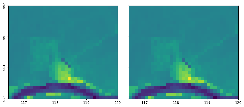
We can plot variables on a map using nlmod.plot.data_array(). We can also use the PlotMapView-class from flopy, and plot an array using the plot_array method.
f, ax = nlmod.plot.get_map(ds.extent, ncols=2)

# plot using nlmod
pc = nlmod.plot.data_array(ds["top"], ds=ds, ax=ax[0])

# plot using flopy
pmv = flopy.plot.PlotMapView(modelgrid=modelgrid, ax=ax[1])
pmv.plot_array(ds["top"])
<matplotlib.collections.PathCollection at 0x769d2290c790>
Cross-sections
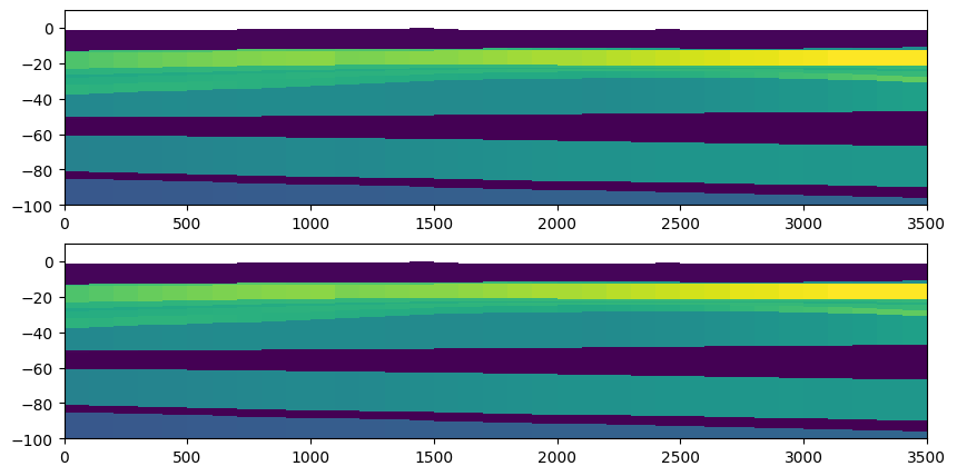
We can also plot cross-sections, either with DatasetCrossSection in nlmod, or using the PlotCrossSection class of flopy.
y = (ds.extent[2] + ds.extent[3]) / 2 + 0.1
line = [(ds.extent[0], y), (ds.extent[1], y)]
zmin = -100.0
zmax = 10.0
f, ax = plt.subplots(figsize=(10, 5), nrows=2)

# plot using nlmod
dcs = DatasetCrossSection(ds, line=line, zmin=zmin, zmax=zmax, ax=ax[0])
dcs.plot_array(ds["kh"])

# plot using flopy
pcs = flopy.plot.PlotCrossSection(modelgrid=modelgrid, line={"line": line}, ax=ax[1])
pcs.plot_array(ds["kh"])
pcs.ax.set_ylim((zmin, zmax));
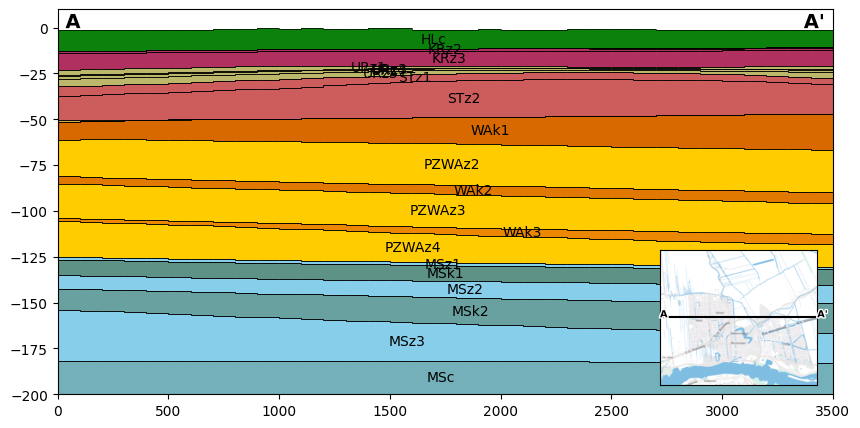
With the DatasetCrossSection in nlmod it is also possible to plot the layers according to the official colors of REGIS, to plot the layer names on the plot, or to plot the model grid in the cross-section. An example is shown in the plot below.
The location of the cross-section and the cross-section labels can be added using nlmod.plot.inset_map() and nlmod.plot.add_xsec_line_and_labels().
f, ax = plt.subplots(figsize=(10, 5))
dcs = DatasetCrossSection(ds, line=line, zmin=-200, zmax=10, ax=ax)
colors = nlmod.read.regis.get_legend()
dcs.plot_layers(colors=colors, min_label_area=1000)
dcs.plot_grid(vertical=False, linewidth=0.5)
mapax = nlmod.plot.inset_map(ax, ds.extent)
nlmod.plot.add_xsec_line_and_labels(line, ax, mapax)
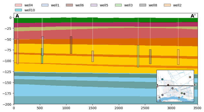
Another feature of the DatasetCrossSection is the plot_wells method to plot the screen depths in a cross section.
# create data frame with well data (random)
nwells = 11
max_dist = 1000
df = pd.DataFrame(
    {
        "screen_top": np.random.randint(-80, -40, nwells),
        "screen_bottom": np.random.randint(-125, -81, nwells),
        "x": np.random.randint(ds.extent[0], ds.extent[1], nwells),
        "y": np.random.randint(ds.extent[2], ds.extent[3], nwells),
    },
    index=[f"well{i}" for i in range(nwells)],
)
cmap = plt.get_cmap("tab20")
df["filtercolor_face"] = [
    cmap(i)
    for i in np.linspace(0, int((len(df) - 1) * cmap.N / len(df)), len(df), dtype=int)
]
df['tubecolor'] = 'white'
gdf = gpd.GeoDataFrame(df, geometry=gpd.points_from_xy(df.x, df.y))

# plot cross section
f, ax = plt.subplots(figsize=(10, 5))
dcs = DatasetCrossSection(ds, line=line, zmin=-200, zmax=10, ax=ax)
colors = nlmod.read.regis.get_legend()
dcs.plot_layers(colors=colors)

# plot wells in cross section
dcs.plot_wells(
    df,
    legend=True,
    max_dist=max_dist,
    filter_patch_kwargs={'alpha':0.5, 'zorder':10},
    filter_rect_kwargs={'alpha':0.5, 'zorder':10},
    tubeline_kwargs={'alpha':0.5},
    legend_kwds={"loc": (0, 1), "frameon": False, "ncol": 7},
)

# inset map
mapax = nlmod.plot.inset_map(ax, ds.extent)

# plot all wells in grey, wells within x meter of cross section in color
gdf.plot(ax=mapax, color="grey", edgecolor="grey", markersize=20)
gdf_plotted = gdf[gdf.geometry.distance(LineString(line)) <= max_dist]
gdf_plotted.plot(
    ax=mapax, color=gdf_plotted["filtercolor_face"], edgecolor="k", markersize=20
)

nlmod.plot.add_xsec_line_and_labels(line, ax, mapax)
INFO:nlmod.plot.dcs.plot_wells:plotting 8 of 11 wells within 1000m of cross section line
Animation
There is also an option to make an animation of a cross section with variations in heads
# make animation of the heads over time
import matplotlib as mpl
import numpy as np

f, ax = plt.subplots(figsize=(15, 5))
dcs = DatasetCrossSection(ds, line=line, zmin=-3.0, zmax=0.0, ax=ax)

dcs.plot_grid(vertical=False, linewidth=0.5)

vmin = np.nanmin(ds["head"])
vmax = np.nanmax(ds["head"])
norm = mpl.colors.Normalize(vmin, vmax)

mapax = nlmod.plot.inset_map(ax, ds.extent)
nlmod.plot.add_xsec_line_and_labels(line, ax, mapax)

plt.close(f)
from IPython.display import HTML

HTML(dcs.animate(ds["head"], head=ds["head"], norm=norm).to_jshtml())
INFO:matplotlib.animation.save:Animation.save using <class 'matplotlib.animation.HTMLWriter'>
Time series
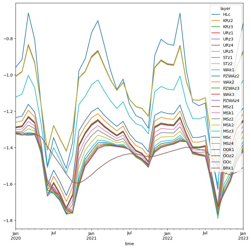
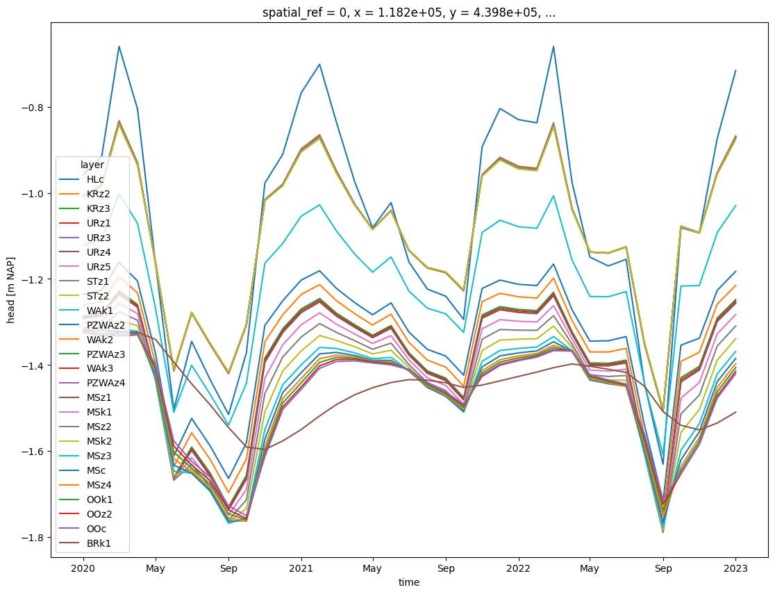
For time series we use the functionality of xarray, as we have read the heads in a xarray DataArray.
x = 118228
y = 439870
head_point = nlmod.gwf.get_head_at_point(ds["head"], x=x, y=y, ds=ds)
head_point.plot.line(hue="layer", size=10);
We can also use pandas to plot the heads. First transform the data to a Pandas DataFrame.
df = head_point.to_pandas()
df
| layer | HLc | KRz2 | KRz3 | URz1 | URz3 | URz4 | URz5 | STz1 | STz2 | WAk1 | ... | MSk1 | MSz2 | MSk2 | MSz3 | MSc | MSz4 | OOk1 | OOz2 | OOc | BRk1 |
|---|---|---|---|---|---|---|---|---|---|---|---|---|---|---|---|---|---|---|---|---|---|
| time | |||||||||||||||||||||
| 2020-01-01 | -0.958394 | -1.006456 | -1.007051 | -1.007532 | -1.007583 | -1.007625 | -1.007717 | -1.008116 | -1.009600 | -1.122572 | ... | -1.302374 | -1.313064 | -1.319242 | -1.325287 | -1.325266 | -1.323120 | -1.320814 | -1.318473 | -1.318109 | -1.317438 |
| 2020-02-01 | -0.915107 | -0.981147 | -0.981961 | -0.982585 | -0.982651 | -0.982706 | -0.982827 | -0.983358 | -0.985274 | -1.105886 | ... | -1.298786 | -1.311698 | -1.321009 | -1.330239 | -1.332089 | -1.331498 | -1.329895 | -1.328345 | -1.327653 | -1.319673 |
| 2020-03-01 | -0.659881 | -0.832225 | -0.834327 | -0.835792 | -0.835951 | -0.836081 | -0.836373 | -0.837683 | -0.842124 | -1.002406 | ... | -1.255993 | -1.276507 | -1.296395 | -1.316075 | -1.324473 | -1.329322 | -1.330917 | -1.332494 | -1.332200 | -1.322446 |
| 2020-04-01 | -0.805093 | -0.929260 | -0.930777 | -0.931854 | -0.931970 | -0.932065 | -0.932278 | -0.933226 | -0.936476 | -1.070815 | ... | -1.280757 | -1.295857 | -1.308574 | -1.321377 | -1.326133 | -1.328325 | -1.329075 | -1.329852 | -1.329741 | -1.324160 |
| 2020-05-01 | -1.161230 | -1.160665 | -1.160671 | -1.160766 | -1.160775 | -1.160782 | -1.160796 | -1.160840 | -1.161197 | -1.266124 | ... | -1.429208 | -1.434681 | -1.432018 | -1.430201 | -1.424022 | -1.416465 | -1.409062 | -1.402345 | -1.398121 | -1.340232 |
| 2020-06-01 | -1.502846 | -1.414051 | -1.412990 | -1.412401 | -1.412335 | -1.412281 | -1.412157 | -1.411577 | -1.409992 | -1.509927 | ... | -1.666293 | -1.667700 | -1.656237 | -1.646332 | -1.632602 | -1.617631 | -1.602161 | -1.588306 | -1.576637 | -1.393135 |
| 2020-07-01 | -1.345041 | -1.279720 | -1.278946 | -1.278558 | -1.278514 | -1.278478 | -1.278395 | -1.277998 | -1.277025 | -1.400485 | ... | -1.614523 | -1.630724 | -1.641150 | -1.651370 | -1.651194 | -1.647081 | -1.639647 | -1.632436 | -1.623803 | -1.443659 |
| 2020-08-01 | -1.433921 | -1.352278 | -1.351306 | -1.350790 | -1.350733 | -1.350685 | -1.350576 | -1.350061 | -1.348719 | -1.467901 | ... | -1.670450 | -1.683163 | -1.688226 | -1.693535 | -1.690524 | -1.684289 | -1.676239 | -1.668437 | -1.660413 | -1.492440 |
| 2020-09-01 | -1.514813 | -1.420354 | -1.419228 | -1.418613 | -1.418545 | -1.418488 | -1.418360 | -1.417757 | -1.416151 | -1.539468 | ... | -1.748448 | -1.760684 | -1.764053 | -1.767908 | -1.763320 | -1.755502 | -1.745762 | -1.736549 | -1.727329 | -1.545339 |
| 2020-10-01 | -1.371344 | -1.306941 | -1.306179 | -1.305809 | -1.305767 | -1.305732 | -1.305653 | -1.305272 | -1.304382 | -1.442472 | ... | -1.689073 | -1.712815 | -1.733652 | -1.754280 | -1.761004 | -1.762773 | -1.759715 | -1.756698 | -1.749818 | -1.590486 |
| 2020-11-01 | -0.977541 | -1.015694 | -1.016174 | -1.016601 | -1.016646 | -1.016683 | -1.016765 | -1.017117 | -1.018520 | -1.163604 | ... | -1.430489 | -1.466326 | -1.508664 | -1.549507 | -1.572499 | -1.589270 | -1.600395 | -1.610166 | -1.612922 | -1.596198 |
| 2020-12-01 | -0.910777 | -0.979810 | -0.980662 | -0.981317 | -0.981387 | -0.981445 | -0.981573 | -0.982134 | -0.984170 | -1.117633 | ... | -1.352868 | -1.381266 | -1.413863 | -1.445778 | -1.463874 | -1.477493 | -1.487911 | -1.497371 | -1.503172 | -1.576365 |
| 2021-01-01 | -0.768087 | -0.897831 | -0.899417 | -0.900547 | -0.900669 | -0.900769 | -0.900993 | -0.901993 | -0.905438 | -1.054387 | ... | -1.306625 | -1.335002 | -1.367514 | -1.399816 | -1.417796 | -1.431535 | -1.441364 | -1.450852 | -1.456353 | -1.549864 |
| 2021-02-01 | -0.701431 | -0.864775 | -0.866768 | -0.868159 | -0.868309 | -0.868432 | -0.868709 | -0.869948 | -0.874153 | -1.028021 | ... | -1.278598 | -1.303755 | -1.331494 | -1.359098 | -1.374072 | -1.385308 | -1.393739 | -1.401810 | -1.407790 | -1.518163 |
| 2021-03-01 | -0.835059 | -0.947943 | -0.949324 | -0.950312 | -0.950418 | -0.950505 | -0.950700 | -0.951567 | -0.954559 | -1.088276 | ... | -1.305002 | -1.323993 | -1.342720 | -1.361569 | -1.370784 | -1.377209 | -1.382224 | -1.387184 | -1.391879 | -1.491979 |
| 2021-04-01 | -0.974722 | -1.026291 | -1.026928 | -1.027433 | -1.027486 | -1.027530 | -1.027627 | -1.028047 | -1.029593 | -1.142460 | ... | -1.328039 | -1.343637 | -1.357625 | -1.371761 | -1.377777 | -1.381381 | -1.384198 | -1.387048 | -1.390391 | -1.469030 |
| 2021-05-01 | -1.081077 | -1.084913 | -1.084972 | -1.085103 | -1.085115 | -1.085125 | -1.085146 | -1.085220 | -1.085655 | -1.184476 | ... | -1.349877 | -1.363327 | -1.374172 | -1.385180 | -1.389021 | -1.390670 | -1.391842 | -1.393142 | -1.395363 | -1.452706 |
| 2021-06-01 | -1.022843 | -1.040828 | -1.041060 | -1.041306 | -1.041331 | -1.041352 | -1.041396 | -1.041578 | -1.042369 | -1.149078 | ... | -1.331847 | -1.349169 | -1.365694 | -1.382194 | -1.389276 | -1.393489 | -1.395734 | -1.398027 | -1.399757 | -1.440687 |
| 2021-07-01 | -1.160642 | -1.134248 | -1.133942 | -1.133839 | -1.133826 | -1.133815 | -1.133789 | -1.133648 | -1.133402 | -1.228249 | ... | -1.387803 | -1.398939 | -1.405840 | -1.412976 | -1.413828 | -1.412639 | -1.411310 | -1.410129 | -1.410614 | -1.433889 |
| 2021-08-01 | -1.223576 | -1.174772 | -1.174195 | -1.173921 | -1.173890 | -1.173863 | -1.173803 | -1.173504 | -1.172771 | -1.268044 | ... | -1.429911 | -1.440700 | -1.446341 | -1.452196 | -1.451524 | -1.448684 | -1.445414 | -1.442423 | -1.441278 | -1.435326 |
| 2021-09-01 | -1.240331 | -1.185818 | -1.185173 | -1.184858 | -1.184822 | -1.184792 | -1.184722 | -1.184386 | -1.183538 | -1.281270 | ... | -1.447890 | -1.459506 | -1.466054 | -1.472688 | -1.472517 | -1.469956 | -1.466905 | -1.464050 | -1.462488 | -1.441273 |
| 2021-10-01 | -1.294222 | -1.228252 | -1.227468 | -1.227065 | -1.227019 | -1.226981 | -1.226894 | -1.226478 | -1.225386 | -1.324318 | ... | -1.491448 | -1.501659 | -1.505521 | -1.509601 | -1.507385 | -1.502909 | -1.498224 | -1.493814 | -1.491234 | -1.452066 |
| 2021-11-01 | -0.893009 | -0.957571 | -0.958369 | -0.958991 | -0.959058 | -0.959112 | -0.959233 | -0.959764 | -0.961706 | -1.092412 | ... | -1.315885 | -1.340085 | -1.366200 | -1.391400 | -1.404454 | -1.413346 | -1.419289 | -1.424605 | -1.427003 | -1.446605 |
| 2021-12-01 | -0.804181 | -0.917338 | -0.918723 | -0.919722 | -0.919829 | -0.919918 | -0.920115 | -0.920993 | -0.924037 | -1.063641 | ... | -1.294609 | -1.317561 | -1.342018 | -1.366397 | -1.378775 | -1.387522 | -1.393056 | -1.398386 | -1.400836 | -1.436815 |
| 2022-01-01 | -0.830129 | -0.938292 | -0.939616 | -0.940570 | -0.940673 | -0.940757 | -0.940945 | -0.941781 | -0.944682 | -1.078808 | ... | -1.298384 | -1.318997 | -1.340153 | -1.361419 | -1.371839 | -1.379016 | -1.383505 | -1.387962 | -1.390054 | -1.426495 |
| 2022-02-01 | -0.837479 | -0.942722 | -0.944011 | -0.944942 | -0.945042 | -0.945124 | -0.945308 | -0.946122 | -0.948949 | -1.082429 | ... | -1.300006 | -1.319513 | -1.338867 | -1.358271 | -1.367273 | -1.373132 | -1.376541 | -1.379897 | -1.381730 | -1.416436 |
| 2022-03-01 | -0.660278 | -0.837029 | -0.839184 | -0.840681 | -0.840843 | -0.840976 | -0.841275 | -0.842614 | -0.847141 | -1.006777 | ... | -1.262116 | -1.285317 | -1.309623 | -1.333784 | -1.345802 | -1.354128 | -1.359245 | -1.364227 | -1.366592 | -1.406186 |
| 2022-04-01 | -0.975609 | -1.035892 | -1.036635 | -1.037207 | -1.037268 | -1.037318 | -1.037429 | -1.037911 | -1.039658 | -1.155485 | ... | -1.339359 | -1.351064 | -1.358752 | -1.366726 | -1.368249 | -1.367730 | -1.367248 | -1.366881 | -1.367906 | -1.397478 |
| 2022-05-01 | -1.149387 | -1.137637 | -1.137508 | -1.137520 | -1.137519 | -1.137519 | -1.137516 | -1.137481 | -1.137585 | -1.240861 | ... | -1.411631 | -1.422595 | -1.428491 | -1.434875 | -1.434341 | -1.431668 | -1.427944 | -1.424744 | -1.422597 | -1.402849 |
| 2022-06-01 | -1.169869 | -1.140281 | -1.139937 | -1.139814 | -1.139799 | -1.139786 | -1.139756 | -1.139596 | -1.139306 | -1.241428 | ... | -1.414262 | -1.426690 | -1.434695 | -1.442671 | -1.443376 | -1.441559 | -1.438872 | -1.436258 | -1.434734 | -1.409859 |
| 2022-07-01 | -1.154531 | -1.125880 | -1.125548 | -1.125435 | -1.125421 | -1.125409 | -1.125381 | -1.125231 | -1.124976 | -1.229387 | ... | -1.409685 | -1.424266 | -1.435472 | -1.446584 | -1.449265 | -1.449084 | -1.447333 | -1.445619 | -1.444176 | -1.417324 |
| 2022-08-01 | -1.444967 | -1.353646 | -1.352555 | -1.351949 | -1.351882 | -1.351826 | -1.351698 | -1.351099 | -1.349439 | -1.445059 | ... | -1.603578 | -1.609763 | -1.606707 | -1.604850 | -1.597429 | -1.588255 | -1.578108 | -1.569025 | -1.561676 | -1.449613 |
| 2022-09-01 | -1.630583 | -1.507581 | -1.506108 | -1.505262 | -1.505169 | -1.505091 | -1.504916 | -1.504101 | -1.501805 | -1.608278 | ... | -1.784216 | -1.789403 | -1.782482 | -1.776735 | -1.765302 | -1.751784 | -1.737028 | -1.723560 | -1.711636 | -1.508301 |
| 2022-10-01 | -1.080992 | -1.077759 | -1.077738 | -1.077844 | -1.077854 | -1.077862 | -1.077879 | -1.077934 | -1.078395 | -1.216657 | ... | -1.476846 | -1.513504 | -1.556411 | -1.597900 | -1.620404 | -1.636357 | -1.645001 | -1.652937 | -1.650709 | -1.540025 |
| 2022-11-01 | -1.093636 | -1.092852 | -1.092859 | -1.092972 | -1.092983 | -1.092991 | -1.093009 | -1.093068 | -1.093504 | -1.215502 | ... | -1.440742 | -1.469952 | -1.503369 | -1.536552 | -1.554563 | -1.567796 | -1.575861 | -1.583374 | -1.584097 | -1.550536 |
| 2022-12-01 | -0.873788 | -0.952585 | -0.953555 | -0.954287 | -0.954366 | -0.954430 | -0.954574 | -0.955206 | -0.957470 | -1.092315 | ... | -1.327455 | -1.355808 | -1.388502 | -1.420498 | -1.438650 | -1.452257 | -1.462504 | -1.471805 | -1.476950 | -1.534910 |
| 2023-01-01 | -0.715961 | -0.867754 | -0.869607 | -0.870910 | -0.871050 | -0.871166 | -0.871425 | -0.872584 | -0.876538 | -1.029920 | ... | -1.282875 | -1.309336 | -1.338979 | -1.368384 | -1.384631 | -1.396916 | -1.406056 | -1.414789 | -1.420191 | -1.509533 |
37 rows × 26 columns
And then plot this DataFrame.
df.plot(figsize=(10, 10));